| 2011 ASPO-USA Conference: Day 1 | The Oil Drum | Tech Talk: A Review of North American Future Oil Production |
Deepwater GOM: Reserves versus Production - Part 2: Atlantis, Mad Dog & Eugene Island
Posted by Luis de Sousa on November 11, 2011 - 10:45am
This a guest post by Jean Laherrère, a long-time guest contributor to TheOilDrum. Jean thoroughly analyses field production data for the Gulf of Mexico (GOM) in several posts. The goal of this series is to compare the evolution of reserves estimates in the GOM with the actual production figures that show the oil decline, thereby investigating the reliability of reserve estimates. This second installment shall look into the Atlantis, Mad Dog, and Eugene Island fields. The first installment on Thunder Horse & Mars-Ursa can be accessed here.

|
Exploration in the GOM
In the deepwater GOM, BP (in red) has the highest number of discoveries, as shown in this graph from PFC (R.West 2011), particularly with Atlantis and Mad Dog. Shell (in blue) is the second discoverer by number. The cumulative oil and gas discovery displays a typical S curve, but where is the asymptote?
Figure 29: Deepwater (>1000 ft) cumulative discovery from Chevron. |
|
|
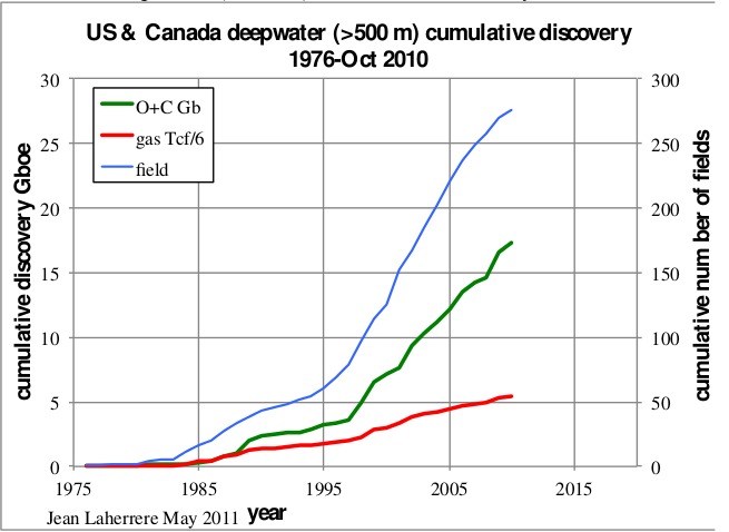
The cumulative deepwater (>500 m) discovery for the US and Canada by the Fall of 2010 was 18 Gb for oil and 30 Tcf for gas.
Figure 30: US and Canada deepwater (>500 m) cumulative discovery. |
|
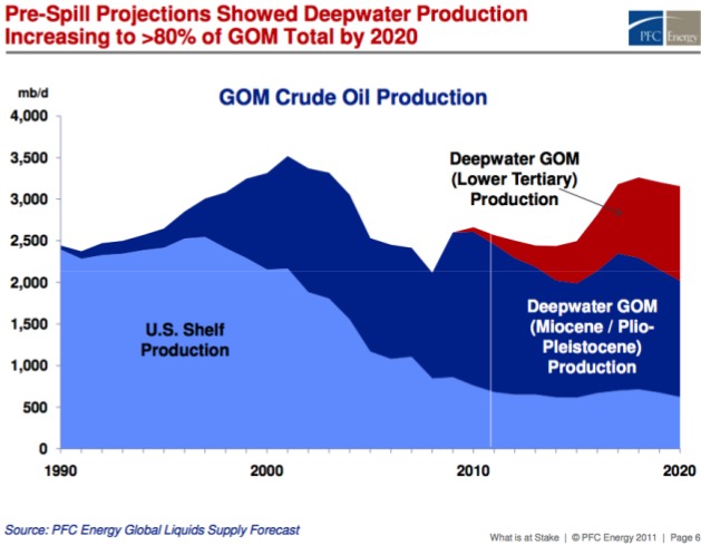
PFC forecasts GOM production to peak again in 2018 due to the Lower Tertiary plays discovered in recent years.
Figure 31: GOM crude oil production from 1990 to 2020 according to PFC. |
|
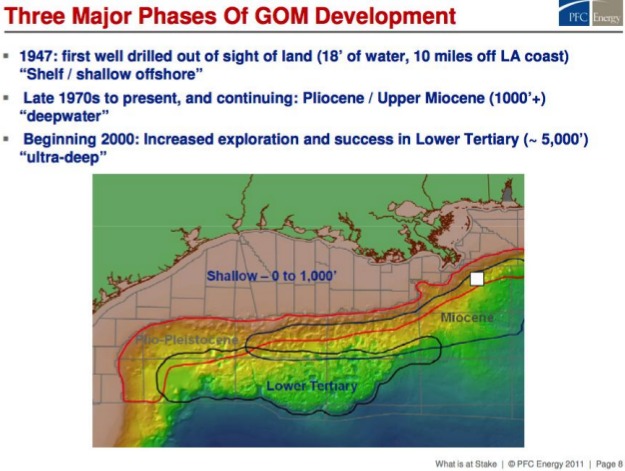
The following map shows the three phases of GOM exploration:
- 1947: shelf-shallow offshore
- late 1990s: Pliocene/Upper Miocene deepwater >1000 ft
- beginning 2000: Lower Tertiary ultra deep >5000 ft
Figure 32: Three major phases of GOM development from PFC. |
|
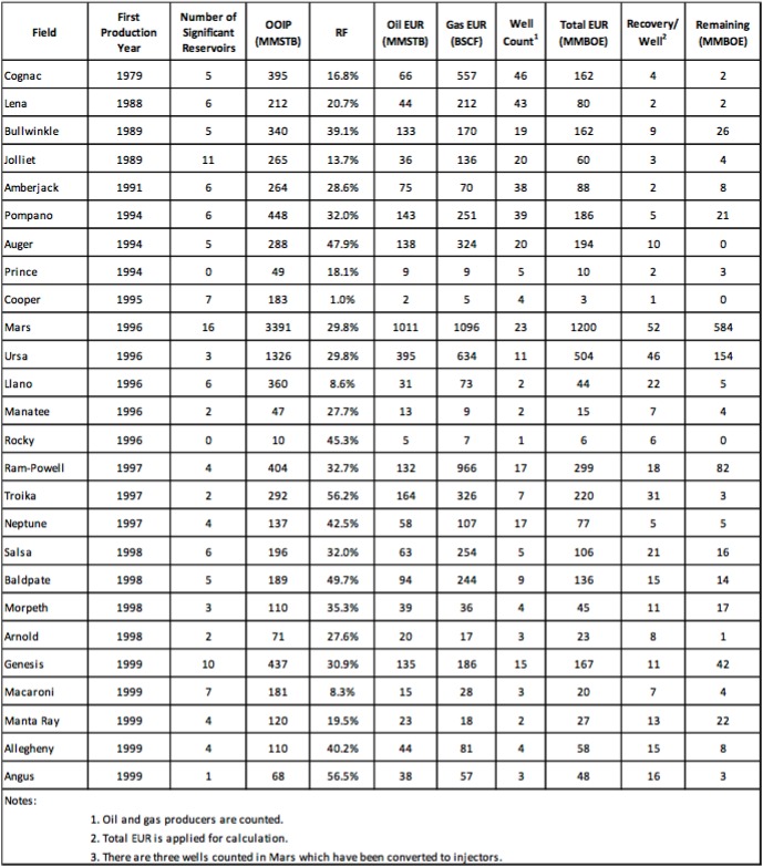
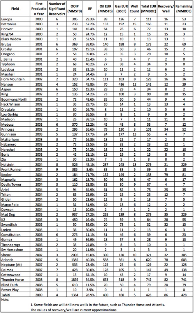
Deepwater reserves (EUR) and oil-in-place (OOIP) are reported by Joseph Lach, Vice President of Reservoir Management in a document titled “Final Report to IOR for Deepwater Gulf of Mexico” published on 15 December 2010.
Figure 33a: Mature fields (1979-1999) deepwater EUR and OOIP from Lach. |
|
Figure 33b: new oil fields (2000-2009) EUR from Lach. |
|
The three significant digits on the recovery factor make me wonder about the understanding of the author on the accuracy of such estimates! OOIP are uncertain figures even at the end of field lifetime; moreover, the accuracy of recovery factors (RF) is about 10%, meaning that only the first digit can be considered as reliable: this is the reason why RF are often reported as rounded (e.g. 30%) or as fraction (e.g. one third).
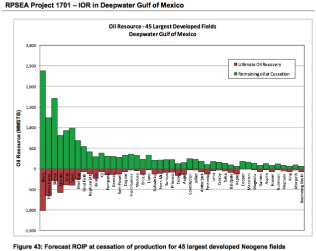
The 45 largest developed fields in the deepwater GOM are reported in a graph also in this document by Lach, showing the ultimate and remaining oil. This graph includes: Mars, Thunder Horse, Shenzi, Atlantis, Ursa, Tahiti and Mad Dog.
Figure 34: GOM deepwater: 45 largest oilfields from Lach. |
|
After Thunder Horse and Mars/Ursa, let's now study other large fields, starting with Atlantis as shown in the next map, operated by BP.
Figure 35: map of the fields developed by BP in the GOM. |
|
|
Atlantis
The Atlantis field (also known as Green Canyon 743) includes in fact the Green Canyon blocks 699, 700, 742, 743, and 744, being located in the Central Gulf of Mexico about 190 miles south of New Orleans, Louisiana. BP and BHP Billiton jointly acquired leases on these blocks under OCS Sale 152 (held on May 10, 1995). BHP retains a 44% working interest in the project with BP being the designated operator. The oil field was discovered in 1998 by the Ocean America semi-submersible, mobile drilling rig operating in a water depth of 1870 metres (6140 ft). The Atlantis platform began production from two wells in October 2007. The Atlantis North Flank began production in July 2009. By 2010, there were twelve wells in production. Twenty wells were originally planned, including 16 producers and four water injection wells.
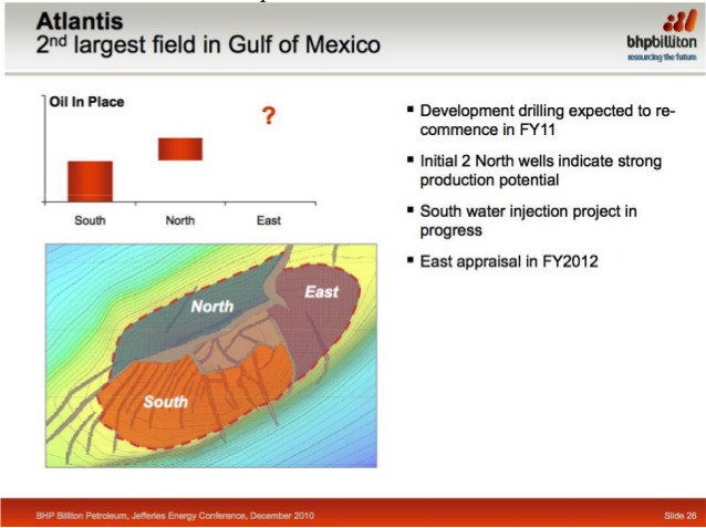
Atlantis is a structure with different compartments. New development will resume in 2011 and in 2012 with the appraisal of the eastern compartment. BHP is presenting more data on Atlantis than BP, the following graphs are taken from a presentation by Michael Yagger to the 2010 Jefferies Energy Conference .
Figure 36: map of Atlantis with its different compartments from BHP. |
|
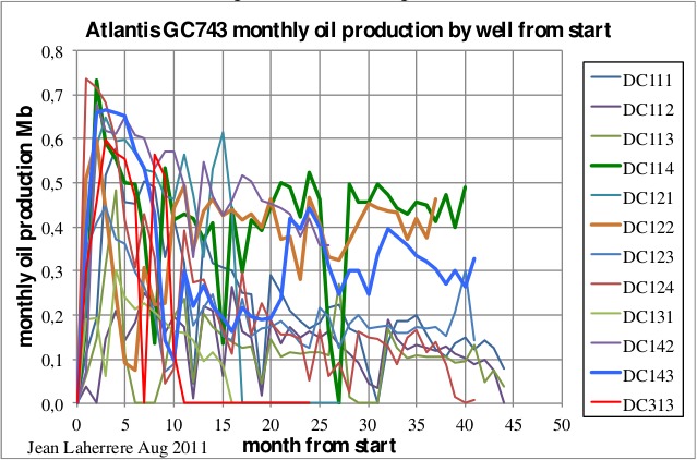
Up to May of 2011 the 12 producing wells display different behaviours in a plot of monthly production from the project start: some decrease, others like DC114 or DC122 do not. In addition to these, well DC102 did not produce anything.
Figure 37: Individual well oil production in the Atlantis field from production start. |
|
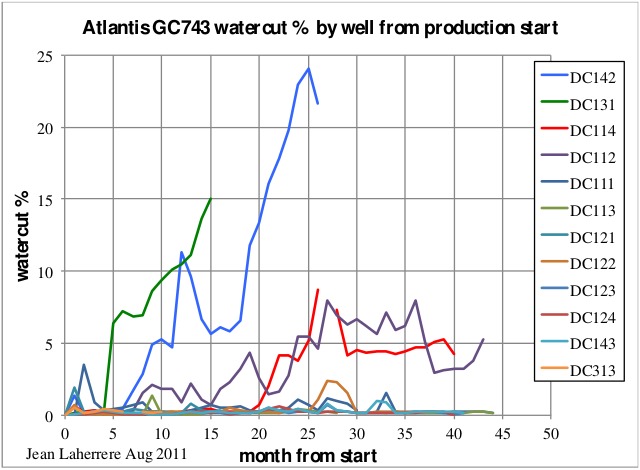
The watercut of those 12 wells behaves also quite differently: DC142 increases to 24% after 25 months; DC131 to 15% after 15 months; DC114 is stable at 5% after 40 months; DC112 went up and down and is now at 5% after 43 months; all other wells have less than 2%. Such low watercut is surprising when looking at the map presented by BHP that shows many faults.
Figure 38: Atlantis individual well watercut from production start. |
|
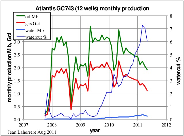
The total monthly production is erratic, but with a decline for oil since May of 2010. The total watercut started increasing sharply from the middle of 2009 but it is still only 7%, which is small when compared to the world average of 75%.
Figure 39: Atlantis monthly production. |
|
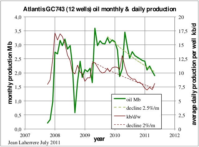
The monthly oil production shows a decline of 2.5% per month since 2010, while the average daily production per well peaked at 18000 b/d in 2008, declined sharply that year and since the middle of 2009 is yielding a slower decline rate, around 2% per month.
Figure 40: Atlantis monthly and daily average per well oil production. |
|
Again, this trend refers to present wells, any new drilling will change the trend.
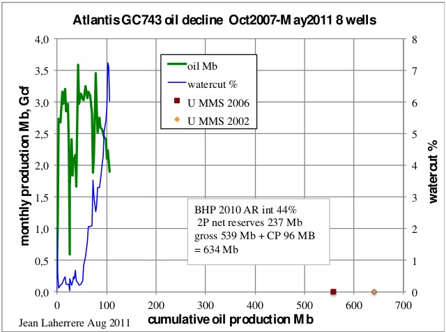
The following graph shows total monthly production versus cumulative production, from which it is hard to extrapolate lacking the plan for future drilling. BP has been very slow to resume drilling after the Macondo blowout when compared to other operators: for the first half of 2011, Shell had 16 drilling permits approved, Chevron had 23, BHP had 15, Exxon has had 11 and BP had none.
Figure 41: Atlantis oil decline. |
|
MMS (now BOEMRE) has estimated the initial reserves in Atlantis at 641 Mb at the end of 2002, but 559 Mb at the end of 2006. BHP in their annual report for 2010 stated their net 2P oil reserves at 237 Mb (from a gross estimate of 539 Mb with a 44% factor for 2P). Adding to this the cumulative production at the end of 2010 of 96 Mb, the initial reserves sum up to 634 Mb. Lach (2010) has an estimated EUR at 558 Mb.
The oil decline can only be extrapolated when all the compartments are drilled and at this time the eastern compartment seems still yet to be drilled. It is thus impossible to say if Atlantis will be a giant oilfield (500 Mb).
Mad Dog
The Mad Dog field, discovered in 1998, is located in the Western Atwater Foldbelt, approximately 190 miles south of New Orleans, USA and is listed by the MMS as GC826. The field is operated by BP, which has a 60.5% share, the remaining stakes belong to BHP Billiton (23.9%) and Chevron (15.6%). The drilling unit is located in 5000 ft to 7000 ft of water in Green Canyon blocks 825, 826 and 782, about 150 miles southwest of Venice, Louisiana. The gross estimated reserves are in the range of 200 to 450 million barrels of oil equivalent. The facility can produce around 80,000 b/d of oil and 60 Mcf/d of natural gas.
A well extending towards the southern region of the field known as “Mad Dog Southwest Ridge" was drilled in March of 2005 and appraised in July of 2009. Drilling results identified around 280 ft of hydrocarbons of Miocene sand and an oil column of over 2200 ft. In 2008 another well, known as A-7, extending towards the western region of the field, identified a hydrocarbon column over 2500 ft with 275 ft of net pay. This field is presently being developed by 12 wells.
The Mississippi fan fold belt is characterised by basinward-verging anticlines and associated thrust faults. Mad Dog is one of a number of discoveries occurring in the western portion of the fold belt, where shallow salt tongues have flown over some of the folds, making seismic imaging difficult.
A seismic profile was shown by Hudec et al (AAPG 2006) as a trap below a salt canopy.
Figure 42: Mad Dog seismic profile. |

|
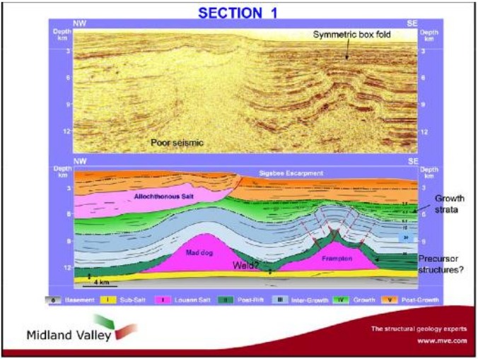
A simplified interpretation was presented by Grando et al (AAPG 2009) as an anticlinal trap above a salt diapir (pink) and below allochthonous salt. The seismic signal below the salt is described as poor!
Figure 43: Mad Dog interpretation by Grando et al. |
|
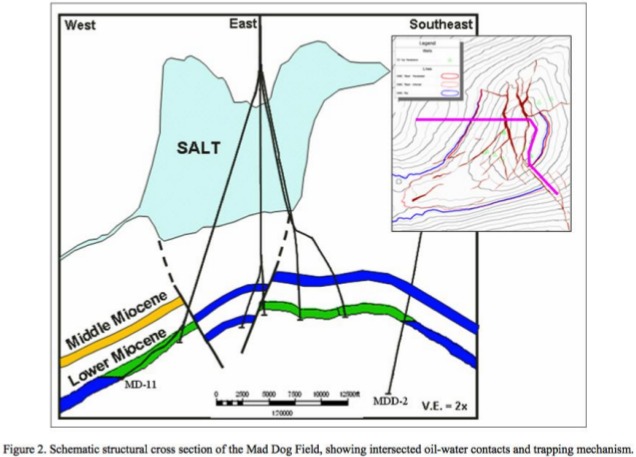
A detailed interpretation of the structure (profile and map) was presented by Dias et al (AAPG 2009). On the profile, the structure is faulted with a wet compartment (graben) in the middle.
Figure 44: Mad Dog cross section from Dias et al. |
|
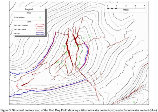
The locations of 14 wells are mapped as tilted (red) and flat (blue) oil-water contacts.
Figure 45: Mad Dog map from Dias et al. |
|
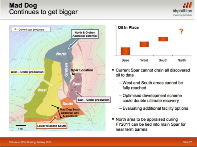
The presentation by Michael Yagger to the 2010 Jefferies Energy Conference shows the potential increase and indicates that the South and West areas of the field are out of reach of the platform presently being used, Spar. The North section of the field is planned to be appraised still in 2011.
Figure 46: Mad Dog map from BHP. |
|
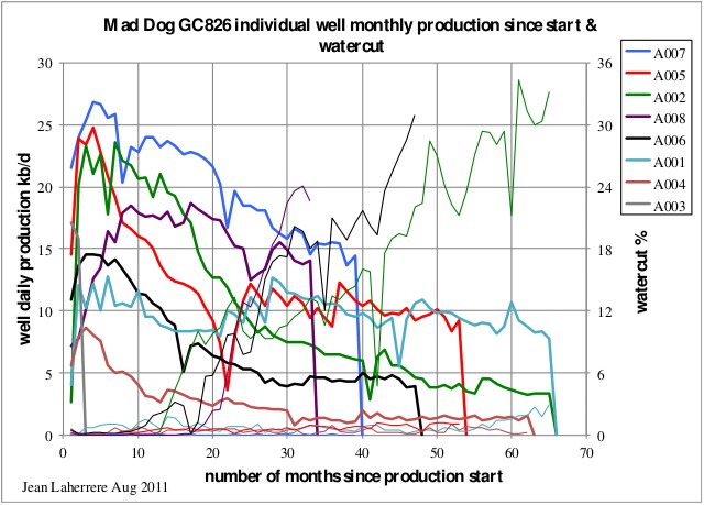
Contrary to Atlantis, the MMS monthly oil production data per well (available for 8 wells) shows decreases in parallel from production start. In some cases the watercut is already over 30% after 50 to 60 months of production, but for the majority of the wells it has remained very low.
Figure 47: Mad Dog individual well monthly oil production and watercut. |
|
The total monthly production for oil, gas and water with the total number of production days shows an increase from 2005 to the peak at the beginning of 2009. Discounting the quasi-annual stoppages for maintenance, the decline is almost symmetrical to the rise.
Figure 48: Mad Dog monthly production from 8 wells and number of production days. |

|
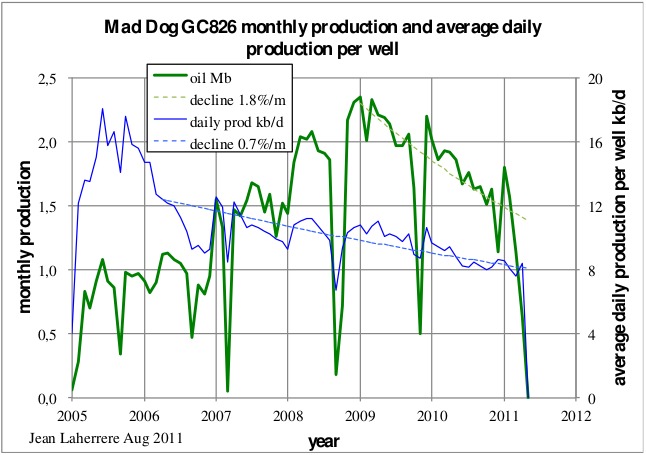
Following is a plot of monthly oil production, which peaked in January of 2009 at 2.3 Mb/m, together with the average daily production per well, which peaked at 17,000 b/d by the middle of 2005. Monthly oil total production declines at about 1.8% per month; when the average daily production per well declines at only 0.7% per month.
Figure 49: Mad Dog monthly oil production and average daily production per well. |
|
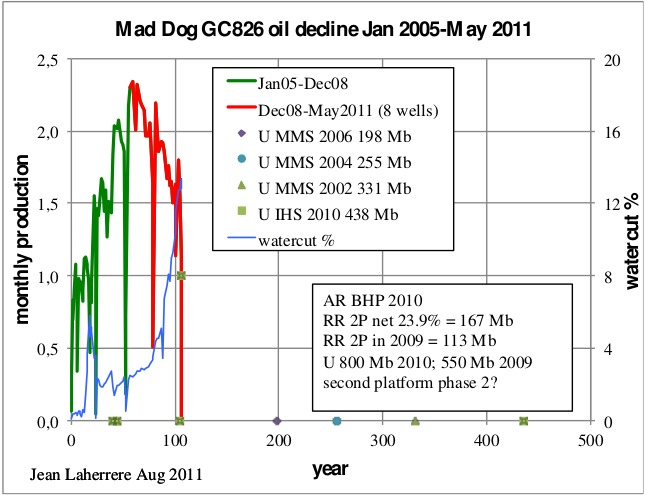
The next graph shows monthly oil production versus the cumulative production, with the various ultimate estimates. It is amazing to see MMS estimates decreasing from 2002 at 331 Mb to 2006 at 198 Mb, while BHP claims initial reserves around 800 Mb (167 Mb net + 101 Mb cum prod) in 2010, with a sharp increase from their 2009 estimate of 550 Mb (113 Mb net + 80 Mb cum prod). In 2010 IHS estimated the ultimate to be 438 Mb (up from 255 Mb in 2004, 195 Mb in 2003 and 193 Mb in 1999). Also in 2010, Lach reported the ultimate at 255 Mb.
It will be interesting to see the next BOEMRE oil and gas reserves estimate for the of end 2007. Past production cannot yet tell which ultimate is right, because the full filed structure is not yet completely appraised!
Figure 50: Mad Dog oil decline. |
|
Eugene Island 330 (EI330)
Back in December of 2003, I gave a presentation "How to estimate future oil supply and oil demand?" at Copenhagen to the International Conference on Oil Demand, Production and Costs - Prospects for the Future, organized by the Danish Technology Council and the Danish Society of Engineers. In it I studied the oil depletion at the end of 2000 of several oil fields in the GOM: EI330, WD030 and SP027. It is interesting to update those three fields.
This Eugene Island field is famous because of a 1999 Wall Street Journal (WSJ) article that started a controversy about its oil depletion rate because of refilling from a deeper source. Astronomer T. Gold claimed this was proof of an abiogenic nature to oil, originating in the Earth's mantle, and that EI330 also explained the large increase (300 Gb) in OPEC reserves during the second half of the 1980s (due in fact to their fight on quotas).
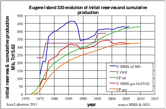
EI330 was discovered in December of 1971 by Pennzoil and Shell in shallow water (247 ft) and production started in September of the following year. In 1983, up to nine platforms were installed. Production peaked around 100,000 b/d in 1976 for a short period of time; during that year EI330 was the largest offshore oil producer with 31 Mb. But it declined sharply afterwards, at 2% per month up to 1983; this decline then slowed to less than 1% per month up to 1992, when the production started to increase to a new peak in 1996, when the mystery of EI330 made it to the newspapers. The WSJ was wrong by stating that “the reserves have rocketed to more than 400 Mb from 60 Mb”. Initial reserves estimates by the MMS were 120 Mb in 1975, 460 Mb in 1986, 350 Mb in 1989 and 410 Mb in 1996; it is difficult to see a rocket - it is behaving more like a drunk fly.
The following graph shows this evolution for oil and gas ultimate reserves estimated by the MMS and the OGJ, plus cumulative production. No mystery, except that the MMS reserve estimate was chaotic!
Figure 51: EI330 evolution of initial reserves and cumulative production. |
|
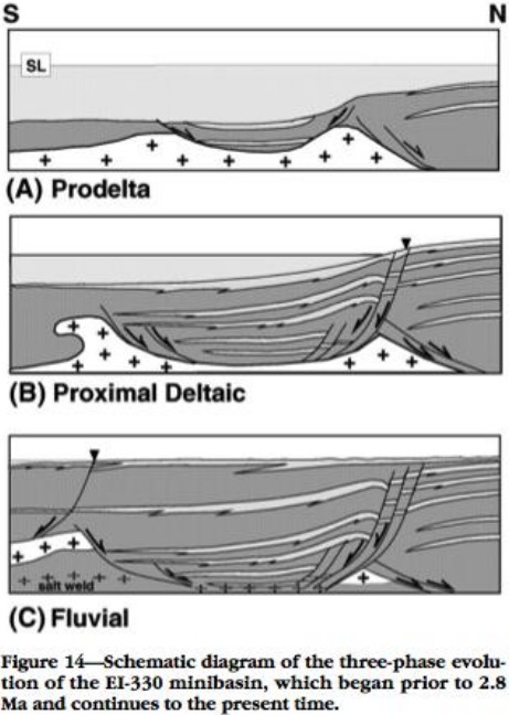
The explanation of the mystery on this production increase is geological. The EI330 trap is against one of the largest faults in the GOM. After considerable production, the pressure, which is typically huge in these Plio-Pleistocene reservoirs, dropped to a point where it allowed refilling from the source-rock, with which these reservoirs are in direct communication. The migration between source-rock and the trap usually takes a long time: here the assumed refilling starting in 1992 was quick (few years) in geological time.
In a presentation entitled “Oil and gas: what future?” delivered at Groningen in the 21st of November of 2006 I wrote:
There is another example of exceptional positive reserve growth, which is Eugene Island 330 in the Gulf of Mexico. The largest fault in the area called the Red Fault (studied on the web by several universities) allows the reservoir to be directly in communication to the source rock and when the pressure dropped the reservoir was fairly quickly recharged by the source-rock. In 1999, Wall Street Journal (Cooper) stated from this example that oil was coming from the mantle, making oil renewable and almost unlimited.
Figure 11: Oil decline of Eugene Island 330 (US Gulf of Mexico) 1972-2003.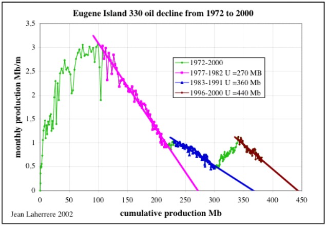
An MSc thesis by B.B. Stump (Pennsylvania State University, December 1998) studied over pressures in some EO330 reservoirs. Laurel L. Alexander and Peter B. Flemings in “Geologic Evolution of a Pliocene–Pleistocene Salt-Withdrawal Minibasin: Eugene Island Block 330, Offshore Louisiana” (AAPG Dec 1995 v79 n°12 p1737-1756) explain the formation of the EI330 reservoirs and respective trap, with this large fault.
Figure 52: EI330 schematic diagram on the evolution of the three geological phases. |
|
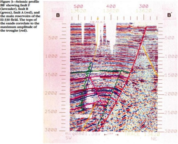
In the AAPG of March 1998, the same L.L. Alexander displays a seismic profile with the A fault (in red), which goes from the deep towards the surface.
Figure 53: EI330 seismic profile with the A fault (in red). |
|
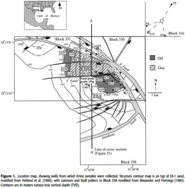
The following map is from “Reservoir fluids and their migration into the South Eugene Island Block 330 reservoirs, offshore Louisiana” by Steven Losh et al. EI330 is also called South Eugene Island block 330 (SEI330).
Figure 54: EI330 structure map on sand OI-1. |
|
In 2004, EI330 was studied to be used for CO2 sequestration (M.D.Zoback et al).
Figure 55: GOM infrastructure with EI330 (SEI330) in 2000 (red = oil pipeline, green = gas pipeline). |
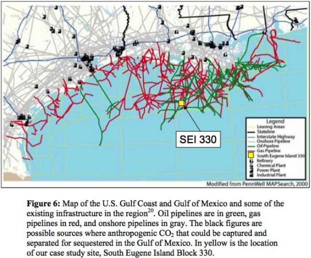
|
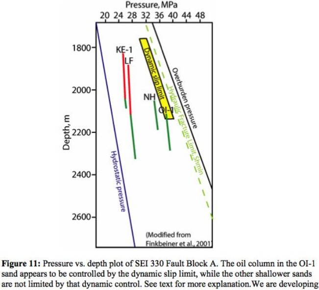
The following diagram shows the pressure of some reservoirs between the overburden and hydrostatic pressure.
Figure 56: EI330 pressure diagram. |
|
This explains that when a reservoir is depleted, lowering the pressure and the resulting lack of pressure, it attracts the migration and recharge of oil through the A fault from the deep source–rock to the reservoir. But the present data shows that the recharge was limited.
The compilation of every GOM field production is given by MMS in their estimate of oil and gas reserves, but the last report is dated of 2009, reporting up to the end of 2006. As mentioned in part 1, I went to the BOEMRE site where there are several (3) reports by unit or per lease and used the shorter one (per unit) which reports only monthly oil, gas and water production by field. But for EI330 I got for 2006 unit monthly oil production ten times less than from the reserves data. To find the source of this discrepancy I went to the production per lease, which details the production broken down into crude oil and condensate (also gas-well gas and casing gas) and I found that the per unit data reports only a part of the data. For example, for 201001, lease G02115 the total for the month of January:
- unit file in page 837 reports only one well (B015) with 149 b for oil and 0 b for water;
- lease file PBOGORAL in page 1834 reports 30 wells with a total of 15 915 b for oil, 145 907 kcf for gas and 90 443 b for water;
- production file PBP9152A in page 1243 reports 20 wells with 15 766 b for oil, 149 b for condensate, 129 268 kcf for gas-well gas, 16 639 kcf for casing gas and 90 443 b for water.
The unit file is incomplete and provides wrong data. I was obliged to go to the OGORA file, which is much more voluminous (5031 pages for 2006 in pdf).
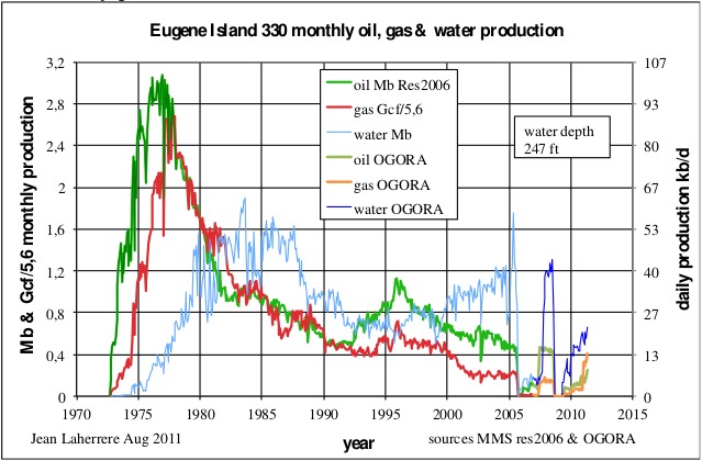
The monthly oil, gas, and water production displays the two oil peaks in 1976 and 1996, with a collapse in 2005 with Katrina, followed by a recovery!
Figure 57: EI330 monthly production. |
|
The monthly oil production versus cumulative production shows that the field is close to depletion and that the initial reserves estimated by the MMS in 2006 could be few MB too short, but their 1986 estimate is likely too high.
Figure 58: EI330 oil decline, watercut and ultimates. |

|
The more recent data (from OGORA) also allows to plot the average daily production per well from 2007 up to now; the decline is from 200 b/d/w in 2007 to about 100 b/d/w today, which is circa 2%/month.
Figure 59: EI330 average daily production per well. |

|
This field will likely be abandoned in the next few years.
A third installment shall conclude this series in the following days.
Deepwater GOM: Reserves versus Production - Part 2: Atlantis, Mad Dog & Eugene Island
PDF version
23 comments
Deepwater GOM: Reserves versus Production - Part 2: Atlantis, Mad Dog & Eugene Island
PDF version
23 comments
Contact
- Content: editors at theoildrum dot com
- Tech support: support at theoildrum dot com
License

This work is licensed under a Creative Commons Attribution-Share Alike 3.0 United States License.
Luis - An outstanding piece. Back in 1975 when I started at Mobil Oil we were developing our portion of the field. One of our best hands was doing the geologic evaluation. He made an amazing statement one day: every time he drilled a new well it proved his current interpretation was WRONG. But most wells found commercial pay anyway. Complex geology to say the least.
Not a criticism but might you expand on the subject of "source rock" for the rest of the TODsters. Other than the obvious I've never seen an official definition for that term. But in general to most in the oil patch it refers to the organic rich shales in which oil (or it's precursor) was created.
Today such source rocks would be similar to the current fractured shale plays being developed. Despite the common misconception that the oil/NG is being produced from those shale rocks, it isn't. The production is coming out of the fractures (cracks) in the shale. The ability of oil/NG to flow out of the shale rock matrix itself is completely insignificant. This is the prime reason such plays are called "unconventional" . There is no reservoir per se in a "conventional" sense. Each "shale well" is producing from those fractures it penetrated as well as other fractures reached by the frac job. So in one sense each well is its own field. Thus one could deplete two such wells in close proximity to each other and then drill a successful well between them and discover "virgin" production.
I've never done a detailed study of EI 330 but that doesn't prevent me from having a theory on the origin of the recharge source. One is quite simple and I've seen examples of before: secondary migration. As the reservoir depletes and pressures drop oil from other portions of the reservoir (that are not being produced by other wells) migrate to the producing wells via the fault/fracture system. My second thought follows your discussion of pressure drop allowing the fault system to open up. It's important for folks to understand the difference between a fault and a fracture. All faults are fractures where there has been movement in opposite direction on either side of the fracture/fault. A fracture is just a fault along which there has been no movement. My next guess is that the recharge oil is draining from various fractures connected to the Mother of All Fractures: the big Red Fault. Think of the Red Fault like one of the massive frac jobs done to a shale play well...except many times more effective. BTW some years ago Shell Oil(?)intentionally drilled into the fault and made a completion. It produced for a bit but as the pressure dropped the fault pinched tight and production ceased. I heard they were contemplating drilling a horizontal well in the fault plane but don't know if they ever tried it. There was a display of EI 330 at the Houston Museum of Nat Science some years ago.
As far as proof of abiotic oil we've beaten that horse to death on TOD. But one last shot: I'll ignore all the other arguments against aboil and ask those folks a simple question: if the mantle is the source of the recharge oil at EI 330 and represents an unlimited supply then why is the field nearly depleted? Oh...oh...oh....I know: aboil is also a finite source and EI 330 has depleted that source. So yes...aboil is real but unfortunately we are way past Peak Aboil.
"Devonian shale gas reservoirs typically are characterized by a low-storage, high flow capacity natural fracture system fed by a high storage, low capacity rock matrix."
SPE #9397
and don't even get me started on sorbed gas......
Examples ?
Yours anecdote seems to be the exception. Operators in the ND Bakken oil play are finding that many (offset) laterals are filled with sand from frac jobs on nearby wells.
Slawson Operating Company lost a drill string, mud motor and mwd, stuck in place with frac sand, while trying to drill a lateral 1/2 mile from another well being frac'ed.
In the Parshall field, EOG resources made an attempt at CO2 huff 'n puff only to find that CO2 showed up in a well more than a mile away within days.
A comparison of performance from the Parshall field with that of the adjoining Sanish field seems to show that more wells only deplete the oil in place faster.
Estimates of 11, or 20 or 24 Gb for the bakken are advocated by public companies trying to convince their gullible flock they can drill 8 wells on a 1280 acre unit. Bexp, soon to be Statoil, suggested they could drill 17 wells on such a unit.
For a discussion of horizontal well interference, see:
Reservoir Characterization of the Bakken Shale From Modeling of Horizontal Well Production Interference Data
http://www.onepetro.org/mslib/app/Preview.do?paperNumber=00024320&societ...
ban - There are tens of thousands of examples in every shale play. At a certain distance from any shale completion there is zero drainage. Which is exactly why we see so much drilling today. If one shale well could drain 2,000 acres obviously they wouldn't be drilling 180 acre units (or less) in many of the plays. Did you notice I didn't quantify the offset distance? It varies with each play. There are always exceptions especially when well spacing is too close. I saw operators in the new Albany Shale have to shut wells in because they frac'd a new well too close and induced N2 in to the production stream of the producing wells...N2 levels exceeded pipeline specs.
The Bakken is somewhat unique in that it appears some of the production is via secondary migration from adjacent sandstone reservoirs. In those cases the fractures in the Bakken extend from those other reservoirs. As far as the rest of the Devonian shale plays I've seen there are no adjacent sandstone reservoirs capable of contributing to recovery.
'Close proximity' is close enough for me. How close is your proximity ? I gave examples of wells drilled 660 feet apart,1/2 mile apart, more than a mile apart and several miles apart(if you dig into Dan Strait's article listed above).
Yes indeed, and the exceptions are the new wells drilled into 'virgin reservoir' in 'close proximity' to other wells.
ban - Think about what the 'exceptions' are. If the majority of shale wells are being drilled into areas being drained by existing wells why are the operators drilling those wells? Do they feel so guilty about their profits they're intentionally p*ssing away money? I can give dozens of examples of wells that drained reservoirs at a long distance. In one case 25 years ago almost 3miles...so what? I can also give examples of wells drilled just a few hundred feet apart that produced from completely seperate reservoirs. In fact, 6 months ago I drilled a well 400' from a pressure depleted well and I'm selling $900,000 of NG/condensate from it every month. Again, what does that have to do with the price of tea in China? We talking about generalities here. And in general shale completions have a very limited drainage radius. Otherwise you wouldn't see the concentration of wells we see being drilled today. Or are you suggesting that the operators who know more about each play than any of us are intentionally drilling too many wells? So all the thousands of new shale wells that have been drilled in recent years and found virgin pressures are the "exceptions"?
Maybe I'm reading you wrong but you appear to be saying that the majority of shale wells being drilled today are tapping into areas already being drained.
The word you are looking for is "designed interference", and it occurs when the NPV calculation encourages it, or the engineering design in an over pressured gas system needs it to solve stimulation thief problems which occur during sequential stimulation jobs, versus doing them all simultaneously. The companies know as well as anyone that long term interference trends won't show up for years in the decline curves of wells in poor permeability rock. The examples listed by Ban are real, and a function of how fracture extension in a particular formation allows long distance communication, versus something slower or more insidious as matrix porosity is drained (and sorbed gas is released) over the longer term.
While a fracture dominated reservoir model may be what you are familiar with in the shales, certainly that is not the only storage system (as you appear to have claimed), and its varying (but unknown) extent allows wells to be drilled close together without problems, or far apart with problems. This variability is why quite a few questions at the most recent SPE national in Denver were centering around the statistical nature of these types of plays, versus the more normal "you can calculate the crap out of all the information" type engineering analysis.
I hear Baker has established a 400-person team to re-evaluate reservoir modeling and production optimization techniques for shale. If this is true, it implies that some major players do not believe their current production approaches, modeling on existing understanding, are adequate.
Any thoughts?
Paleo - I'll check with my Baker rep Monday. But I doubt they have 400 folks working on modeling alone. Maybe a dozen folks in each trend who know what they are doing should suffice. But that number may include all the associated efforts such as frac design. One reason it's complicated is that the geology/fracture distribution is quit variable. The best reservoir model is useless unless the geologic parameters are correctly defined.
Despite all the 'whiz bang' technology being discussed, operators haven't made much progress on efficiently pumping a gassy, 240+ deg F reservoir such as the ND bakken.
I had mused whether expanding gas cools enough to cause problems for oil viscosity. If there is a lot of gas, then there is value in that, though it's a complicating factor for the oil. I guess it's the converse of NGLs being a complication, though valuable, for gas production.
But right now I know production is all about oil, as there is a lot of gas already.
Downhole pumps are designed to pump mainly liquid. If a slug of gas tries to move through the pump, the pump will effectively stall. This leads to excessive wear and pump failure.
High temperature is also a factor in pump wear because of the tight clearances between moving parts for a pump designed to lift from 9,000 feet, as is the case in the ND bakken.
The cooling effect on crude viscosity is not much of a consideration, as the oil, water and rock have a lot of thermal mass and the expansion occurs at an elevated temperature(at pump depth).
Cooling from expanding gas is a major consideration in producing a rich(or not even so rich) gas/condensate. Liquids want to condense and will interfer with the flow of gas through the rock. This occurs mainly in the vicinity of the wellbore.
Paleu - And to add to b's excellent discourse: you may be aware but the cooling effect of gas expansion is so significant we typically put a gas-fired burner on a NG well to heat the production stream. Otherwise the surface flow lines will freeze up and kill the well.
Thanks for the info. The details always get entertainingly complex.
Ponzi. The early player make out like bandits, and the late comers will see what overdevelopment means. I have seen it in conventional and non-conventional plays.
My example is for the ND bakken. There is lots of talk and flashy power point presentations about 8 or 17 wells being drilled in a 1280 acre unit. Yet, the most intensly drilled area of the ND bakken is in Sanish Field which is drilled on an average of about 3 wells per 1280. That field is showing signs of overdevelopment as I mentioned in my original response.
Speak for yourself, I have watched and worked in the bakken play since before the hz play was invented in 1987.
No. I am saying that public traded companies are hyping their 'resource estimates'. I doubt we will see 8 or 17 wells drilled in a 1280 unit.
I have always admired these graphs. I even perused some of the articles in French, just to look at the pictures. I had the opportunity to meet Jean Laherrere at the recent ASPO-USA meeting in Washington DC. Among other things he mentioned that he hopes to see publication of the Second Edition of GeoDestinies by Walter Youngquist
What's the latest on Thunderhorse? (Blunderhorse?)... Google doesn't really bring up nothing new.
Did you see the link to the first installment?
http://www.theoildrum.com/node/8366
I'm too busy nowadays to digest such a long and involved article,not to mention that I am not skilled in interpreting geological maps. I suspect that many more members are in the same situation.
Hopefully somebody who has the time to study it well will post a good summary of this fine piece in the comments section.
RE: Posy (EI 330) Field Recharge
The production profile shows a typical decline with a few bump-ups on the way down.
If you plot #wells drilled per year vs. production you will see that the first production bump up in the early 80's coincides with new wells drilled in reservoirs not initially developed in the 1970s. Also, the big bump up in the mid 90s coincides with the drilling of multiple high-rate horizontal wells in the oil rims and a few undeveloped shallow reservoirs.
I don't know if the fault recharge model ever really convinced the field teams. Reservoirs "overproduce" and "underproduce" on a regular basis - reserves estimates include many important assumptions about aquifer support, thickness and porosity away from well control, structural and stratigraphic complications affecting connectivity. 2P reserves estimates by experts with all the data fluctuate (sometimes disconcertingly wildly) as more data and becomes available, and new development technology is applied.
It's amazing how cornucopians and abiotic crackpots have selectively latched onto one obscure academic study of the possibility of continued oil migration along fault planes in a single field to support their grandiose opinions.
Are there any estimates about the profitability of these endeavors?
I have seen suggestions that no major oil company will take the financial risk of new deep water production development now.
Profitability of individual projects is hard to come by in the public domain.
OTOH, here is a short list of current and announced GOM deep water development projects. Presumably, Exxon, Shell, Chevron, Petrobras, Anadarko, Hess and others and confident that these projects will be profitable.
Telemark (ATP) subsea tiebacks to a MinDoc floating platform
Tubular Bells (Hess) tie backs to a new 3rd party spar
Cardamom (Shell) subsea tieback to existing Auger TLP
Jack/St. Malo development to new FPU (Chevron)
Bigfoot new E-TLP (Chevron)
West Boreas and Deimos South (Shell) subsea tiebacks to...
Mars B (Shell Olympus) new TLP for further Mars field development and host for satellite field tiebacks
Chinook/Cascade FPSO (Petrobras)
Hadrian/Lucius development in system selection phase (Exxon)
As usual, too much data, and not enough statistical synthesis. No one does this kind of bean-counting analysis anymore, especially when you have powerful stochastic techniques that allow the numbers to get rolled up and produce a much more accurate and useful result.