The Shock Model: A Review (Part I)
Posted by Sam Foucher on April 5, 2007 - 9:33am
WebHubbleTelescope, a long time TOD poster, has been one of the most active in the blogosphere in the area of oil production modeling. He has advocated a more physically based approach instead of a heuristic curve fitting approach such as the Hubbert Linearization. He proposed an original method, the so called Shock Model, that has a clear physical interpretation and that is making use of both the production profile and the discovery data. I think that a review of the Shock Model is long overdue.
I also propose three modifications or extensions:
- Originally, the instantaneous extraction rate function E(t) has to be provided by the user. I propose a method to estimate E(t) directly from the observed production profile.
- Reserve growth is modeled as a fourth convolution function based on an empirical parabolic cumulative growth functions (this will be detailed in part II).
- A new way to project future extraction rate (in part II).
In summary, the shock model is a simple and intuitive model that is making use of both the production profile and the discovery curve. In this essay, the method is applied on the world conventional crude oil production (crude oil + condensate) and the ASPO backdated discovery data. Interestingly, the derived Reserve to Production ratio (R/P) seems to match the values obtained when using the proven reserve numbers (BP) once corrected for Middle-East spurious reserve revisions (in 1985, 1988 and 1990). In addition, R/P values are presently at a record low levels and below what have been observed during the previous oil shocks.
The code in R language is provided at the end of this post.
From Discovery to Reserves
The Shock Model is described in details on Mobjectivist. It is based on the following three equations:
The first equation will create reserve additions from the initial discovery numbers (backdated). The second equation is the reserve evolution equation and dictates how reserves will change over time from the cumulative addition of new reserves and consumption. The three filtering functions involved in the computation of the instantaneous reserve addition T(t) are exponential distribution functions:where:
D Discovery (backdated) T Instantaneous gross reserve addition R Oil reserves E Extraction rate or shock function P Annual oil production hBuild,hFallow,hMature Exponential functions
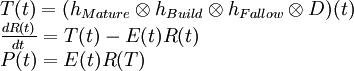
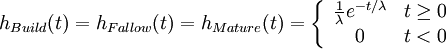
where λ is the mean time period implied by each process. The main reason behind this filtering process is to simulate the different steps (Fallow, Build and Maturation) involved in developing an oil field as shown on Figure 1.
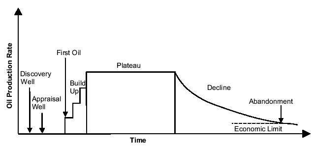
Fig 1. Timeframe for the development of an oil field1 .
The result of the three convolution operations is equivalent to one convolution with a Gamma distribution:
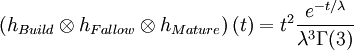
On Figure 2, we can see an original discovery impulse is being spread out on a large time period.

Fig 2. The filtering operation by three successive Exponential distributions is equivalent to a Gamma distribution
The convolution by a Gamma function will smooth and shift the original discovery curve by 2λ. Using the ASPO backdated discovery curve (Figure 3), we get a shifted and smooth reserve curve.

Fig 3. Effect of the succesive convolutions on the original backdated discovery curves (ASPO) .
The question is how to choose a correct value for λ. WebHubbleTelescope is proposing λ=8 years. Higher values for λ will increase the degree of smoothing and the time lag between peak discovery and peak reserves. If you compare the simulated reserve curve with the actual proven reserve numbers (Figure 4), you can see that for λ=3 the reserve curve is matching closely the proven reserve numbers (once corrected for Middle-East increase).

Fig 4. Simulated oil reserves R for different values of λ.
Estimating the shock function
In reality, the extraction rate E is not a constant and presents large fluctuations especially during oil shocks. In WHT's original method, the shock function E(t) is set manually which is not an easy task in my opinion. I propose to estimate the shock function by literally tracking the instantaneous oil production using a bootstrap filter. I have previously applied this technique with good results. In a nutshell, the boostrap filter find the optimal value for E(t) at each time t by stochastically exploring a set of possible values and weighting them according to how well observed production levels are predicted (the technical term is Sequential Importance Resampling or SIR). A result of this approach for λ=3 years is shown on Figure 5, we can see how closely the production levels are reproduced by the model.
Fig 5. World production for crude oil + condensate2.
The figure below is the estimated shock function E(t) with the proposed technique. The shock function is assumed constant in the future and equals to the last estimated value.

Fig 6. Shock function E(t) estimated by the bootstrap filter (with λ= 3 years). Click to enlarge.
Forecasting ability
In my opinion, the model has limited predictive abilities because it cannot predict correctly future extraction rate values (i.e. the shock function E is unknown in the future). WHT has made the following prediction for crude oil + NGL.
Fig 7. World production forecast (crude oil + NGL) .
This forecast includes NGL production which I don't think is appropriate because the model is based on conventional oil discoveries. On Figure 8, we can see the application of the shock model for different time intervals assuming that the extraction rate remains constant in the future and equals to the last estimated value. Predicted production levels are falling immediately because E(t) should increase in order to maintain or increase production. In part II, I will propose a simple solution to deal with this problem.
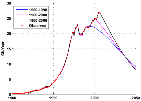
Fig 8. Different world production forecasts for crude oil + condensate .
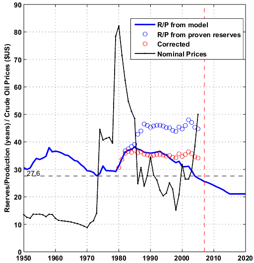
It's interesting to compare the inverse of the estimated extraction rate (1/E(t)), which is equal to the reserve to production ratio (R/P), and fluctuations in nominal crude oil prices:
- When R/P values are below 30 years, prices are increasing. This was the case in 1970 at the time when demand for oil was very strong and energy efficiency not part of the vocabulary. A lowering of consumption after 1985 (mainly a combination of economic slowdown, energy conservation, drilling frenzy,...) has contributed in an increase in the R/P values.
- The recent increase in price since 2003 corresponds also to current R/P values below the 30 years threshold minimum (27.6 years) observed in the 70s.
- The ASPO discovery data is probably underestimating some significant amount of reserve growth that has occured in the late 90s hence the premature fall of the simulated R/P curve around 2000.
- The R/P values given by the model are surprisingly closed to the R/P computed from proven reserves (BP) once corrected from large reserve additions in middle-east countries (red circles).
- In order for the R/P value to come back above 30 years, either reserves need to increase significantly or crude oil consumption needs to decrease significantly.
Fig
9. Crude oil prices are inflation
adjusted (nominal prices). The red dotted vertical line is the year
2007.
In Part II, I will look at the modelisation of reserve growth and a new way to improve the predictive ability of the shock model.
Footnotes:
1Giant oil fields and their importance for future oil production, Fredrik Robelius, PhD Thesis.2The data for the world production of crude oil + condensate is composed of:
- 1900-1959: API Facts and Figures Centennial edition 1959.
- 1960-2006: EIA data.
Code:
The code is available in R language, the windows version of R software is available here. You will need to install the Matlab package (go in "Packages/Install Package(s)" then choose a CRAN site and select Matlab from the package list). To execute the program, open the file given below and click on "Edit/Run all".
Contact
- Content: editors at theoildrum dot com
- Tech support: support at theoildrum dot com
License

This work is licensed under a Creative Commons Attribution-Share Alike 3.0 United States License.
I dedicate this story to Martin Hollinger, a good friend and a great mind, who passed away yesterday.
Wow! I am constantly amazed at the brilliant analysis done here. Thank you WHT and Khebab for your efforts.
I think it is a fair point that if Discovery listed is only for Crude that the Shock may not be appropriate for prediction of C&C. Also the point that some of the listed Discoveries might be reported on the conservative side.
How well does the model work when compared to well know fields that are in decline, (US lower 48, North Sea)?
Thanks again for the brilliant efforts.
Thanks!
Re: ...may not be appropriate for prediction of C&C.
The discovery curve is for C&C.
Re:How well does the model work when compared to well know fields that are in decline, (US lower 48, North Sea)?
It will be the next step, as soon as I can get some discovery datasets.
I agree, excellent work. I was wondering when WHT would be recognized for his efforts.
Interesting stuff. Looking forward to Part II.
I have to go for now, I will answer comments later today.
Khebab, brilliant post. But where is the link to the R code? I did not find a link other than to R itself. Thanks.
See the attachment section at the bottom.
Khebab, sorry, but I don't see any attachment section at the bottom of the post or the comments. There is a "Code" section at the bottom of the post, but it refers to the actual code being down the page somewhere. I don't see that somewhere. Is it possible contributors see an attachment section that the rest of us don't see?
Strange, I will ask our Administrator, here is the link:
http://www.theoildrum.com/files/ShockModel.PartI_.txt
Excellent! Thanks!
Khebab, correct me if I am wrong but I think the oil shock model still has predictive value in that if you extrapolate on current knowns, then shouldn't the resulting picture be the most optimistic scenario possible (i.e. one lacking any further shocks)? So doesn't the oil shock model set upper bounds on what we can expect from production barring further shocks?
Ghawar Is Dying
The greatest shortcoming of the human race is our inability to understand the exponential function. - Dr. Albert Bartlett
The issue is to find a way to extrapolate the model parameters correctly.
Of course, we can't predict future oil shocks (i.e. the predicted curve is smoothed) because the extraction rate is staying constant.
My big problem with the shock model is its tough to prove you have constrained the model enough to be a good predictive. It has to many parameters. Its however a good model for current production and if you feel you have it constrained correctly it probably a good model for the real decline rate post peak.
So I'd like to see how it behaves under further constraints.
A obvious way to introduce further constraints is to use HL as one of the constraints on the model.
Lets assume HL gives two pieces of information that are reasonably accurate.
1.) Maximum total URR.
2.) Minimum or earliest peak date and highest peak production rate.
If HL is wrong and the shock model is at least reasonably predictive you will have obvious disagreements between the two models.
Underlying this assumption is that the URR is a constant and the areas under the two curves are equal with HL representing the theoretical best production model.
By using both approaches and assuming that the shock model is a better fit both for current production and future if constrained I think that we get a better total model.
I'd feel a lot better about the shock model if the constraints where tightened so we know that the parameters are not just better curve fitting.
I don't think HL is required and suspect the additional constraints can be developed using other methods but without them its hard to prove the shock model.
In general the problem is that you need to prove all the inflection points are real and not artifacts of the model.
The more you have in your model the higher the burden of proof needed. So far I don't think this has been done.
I disagree with assumption #1. I have repeatedly read Hubbert's 1956 paper and it is apparent to me that Hubbert did not derive URR. Instead he had pre-existing estimates of URR that he considered as upper and lower bounds - 150GB and 200GB. I have come to the personal conclusion that Deffeyes simplification of Hubbert's technique is erroneous on at least that one count. This does not mean that Hubbert was wrong as he used a different process.
"Hubbert Linearization" was invented by Deffeyes as an attempt to simplify the mathematics of what Hubbert did but Deffeyes apparently leaped to a conclusion that it can predict URR. Instead, I believe that an HL plot can only be valid if it lies within the upper and lower bound of estimated URR for a given producing region.
Ghawar Is Dying
The greatest shortcoming of the human race is our inability to understand the exponential function. - Dr. Albert Bartlett
I agree with GreyZone. In 1956 Hubbert had a range of URR estimates based on his geologic analysis. It was his upper bound that actually turned out to be right for US production. If you haven't read the 1956 paper, do so. It is very interesting.
Hubbert presented the logistic equation later WHT and Deffeyes have documentation on it. I don't disagree with anything you just said. My understanding is the logistic curve was introduced by Hubbert. And yes like any curve fitting method you need at least some reason to thing the data and the model are in rough agreement.
The main point is that the focus should be on the dampening term and in cases where bot HL and shock apply its instructive to understand how the the real term and the empirical term happen to give the same answer.
Its easy enough to throw out HL just takes a small amount of work to correlate the two models. The reason this is important is we have used the empirical HL model a lot we need to show how we moved to a new model. And a bit on why the old one worked.
Its just curve fitting in one case we have a non-physical logistic curve that fits and a better model that fits the data. All you need to do is show the terms in the better model that correlate with the terms in the empirical model.
This can be done with simple parameter variations to show where and when the two models are close.
Another reason to do this is it gives us a better understanding of the physical dampening terms vs the term used in the logistic. Its hard to grok why the logistic one works. And its not obvious what the real term should be.
One problem with the Logistic model is that it's not related to the physical reality of the oil extraction process (which is one of WHT's main argument). It's basically an empirical curve fitting approach that happens to have one of the most easiest fit possible (i.e. a straight line) hence its popularity.
The shock model needs a discovery model to enable it to be used in the same way as the Logistic is used, namely as a self-contained model that uses only discrete parameters but that can fit a URR along with a production curve. The fact that the Logistics model can subsume both a physical discovery model and a physical extraction model at the same time blows my mind. It's almost as if it is too good to be true, and what we will eventually find is that it is indeed too simplistic to be true.
Thus, the effort we put into this analysis.
:)
Funny you say that its fascinating that it seems to work well when used correctly.
To be honest I'm interested in a better model like the shock model simple to see if it sheds some light on why a logistic function seems to work so well for oil production.
Nothing short or brilliant insight would have cause you to choose it for a simple empirical model.
I really wish Hubbert hand explained why.
Short of this we know that at least in some cases a physical model must match the logistic so maybe it will give us some insight.
I have a new theory on the why of the Logistic model. It is called the Theory of Convenience.
http://mobjectivist.blogspot.com/2007/04/how-to-generate-convenience.html
I always thought the Logistic model makes absolutely perfect sense in the context of reproducing biological entities with a constrained food supply. But I can't for the life of me treat oil molecules as reproducing entities unless we replace oil with people as the random variable. And that to me is a scary thought. To paraphrase Soylent Green, "Oil is people!".
Hubbert was very concerned with human population. Hubbert was alive as the Green Revolution kicked off and he surely new that it was powered primarily by fossil fuels.
That's a scary thought, WHT, but what if it is right?
Ghawar Is Dying
The greatest shortcoming of the human race is our inability to understand the exponential function. - Dr. Albert Bartlett
I agree with your analysis in the link what's fascinating is you can get a good fit using HL.
In any case we have examples where the logistic is providing a very good fit. I'd like to see the more realistic shock model applied to the same examples so we can see why the real shock model converges on the hl. You basically have the right answer its hidden in a trick dampening term. But why that form and is it really just a proxy which it should be for the correct dampening term.
Using the shock model you should be able to derive the correct equation that hl just happens to approximate and more important we can find the "real" terms that are the key to this approximation.
I'm happy too throw out HL but you need to show in a few cases where it does work why it worked on the other side this will also show how it fails.
Then we can just dump it.
Hopefully we can shoot it in the head correctly.
But it is pointing to a damping effect that should also arise in the shock model. What I've not seen you do is explain the correlation. So what is the relationship between the correct shock model and the empirical logistic equation.
What in the real model leads to this fudge factor working ?
Thats the one piece I'd like to see once you have that we can dismiss HL and use a better model.
I think this boils down to the non-linear damping term and what does this correlate with in the shock model ?
I don't think the form of the growth term is all that important.
And if you think about it the important piece of all of these model is the dampening effect the growth term can be any form even linear. The shock model seems to give the correct growth side but what exactly is the dampening term and why does the logistic one fit ?
Next you seem to imply a non-linear dampening effect is bad but why ?
To wrap up the growth in production can be modeled fairly well the shock model seems to have the most important parameters whats not well understood is how to model the complex process related to the field geology that result in peak and decline.
The logistic works because of a fudge factor that causes the curve to fit but contains no intrinsic physical interpretation.
At least thats my problem. Its not the growth but the decline
I don't understand. And of course I don't understand the shock model well enough to pull this out. Finally the model presented so far in this thread does not seem to be the right one on the decline side in the first place which is the juicy part :)
Don't agree re:Verhulst, and I'll be schizo about it.
1. I agree that the damping term makes no physical sense, but the source term makes no more sense than the damping term. Oil wells (I'm no expert here, so feel free to correct me) don't breed, so a source term that is proportional to the current number of wells makes no physical sense.
2. OTOH, the Verhulst equation converges to a value which in population dynamics is the maximum sustainable population. Perhaps one really can associate global URR with this limit (which is really what we do when we do HL). One can further stretch the analogy to argue that initial growth is logistic because the more we have, the more uses we find for this magic black goop and the more effort we expend finding the stuff. But eventually diminishing returns hits: fields deplete, new sources become scarce, and we asymptote (big wavy hands here -- in this case the functional form of the damping can be argued) to a limit.
3. OT3H, there is an underlying assumption that changes in production are continuous. Is that reasonable? At fine enough resolution that does not appear to be the case. If the behavior is essentially logistic, whether it is continuous or discretized can make a huge difference. Three possibilities here: a) the system is logistic and continuous; b) the system is logistic and discontinuous but the growth rate is small enough to avoid the chaotic regime; c) the system is not logistic. b) is interesting because that would imply that URR depends on the growth rate (how hard we suck).
I'm not arguing in favor of HL and actually never have.
As a empirical model it works. Any real model will give a similar result which means it probably will have a interesting dampening term. Where both models work my interest in in the nature of the dampening term. Because as you know stated an attempt to match HL to physics is pretty wacked.
On the source side I think thats less important since changing the source function is really just a matter of better curve fitting in the case of the shock model it can be matched to the physical process. I'm not saying its not important in that sense but it the dampening term that leads to peak and decline and at least for HL is a very strange non physical term but since the curve can match real production what is the form of a physical dampening factor that gives the same answer ?
As of now I can only see the matching if the real model has a similar set of conditions as hl but that does not make sense why would something like a logistic function drop out ?
Empirical curve fitting does not require the function to have any physical meaning but when you have such a strange function gives a good fit it makes you wonder what the real model will give.
A post postmortem on the abandoned HL model and why it happens to work is interesting. And I think needed before we abandon the method. The answer may be trivial but its needed to justify abandoning HL.
The flip side is also true if HL is still giving a better fit than a physical model you have to question the physical model. Or on the same hand if you have to add too many parameters to the physical model to make fit you have to question the model.
I don't like the damping term in the Logistic model either but I also don't necessarily like the exponential growth term.
Importantly, the shock model by itself has no growth term, apart from the "growth" from discovery to maturation of individual wells. The actual significant growth occurs in the discovery model, and this has little to do with extraction and more to do with technical prospecting. Note that the shock model assumes a discovery model, albeit in this case based on real data. This is where I marvel/wonder about the Logistic model, in that you cannot factor out a discovery profile along with an extraction profile from such a simple function. Whereas, you can come arbitrarily close to generating a Gaussian by convolving many small ditributions together (i.e. the Central Limit Theorem).
My current conjecture is that discovery follows a power law, most likely a cubic, which comes about by technology increasing the width of a prospecting zone linearly with time over the years. However, this is definitely not an exponentially increasing function.
http://mobjectivist.blogspot.com/2007/03/cubic-growth-discovery-model.html
That curve you see above is the shock model "deconvolved" to show a conjectured original discovery profile dated back to when oil was first discovered.
That makes sense to me. But the logistic is both exponential growth and nonlinear dampening is it exponential I can't tell because you did not integrate it. And I'm too lazy to try.
But to overcome exponential growth you need a exponential decay so I think I'm right just guessing.
My best guess is the model of two competing exponentials happens to result in something similar to what your saying.
The insight is to recognize that oil production results in two competing exponential functions. I don't think this is obvious from a physical model. So the contribution of HL to a physical model is to accept that the model may need to include the concepts of exponential growth and decay.
My guess right now is that growth is not exponential but that decay is but its delayed by a time constant before it sets in. The exponential growth part of HL is not important and its swamped by the decay term later and when it is in force the difference between a exponential and cubic etc is small. It just acts to fudge the lack of time delay in the decay function.
So the real model is a none exponential growth curve that gets obliterated when exponential decay sets in the decay is offset in time.
The reason decay is exponential goes back to Fractional Flows
With fractional flow diagrams you get catastrophic failure this step function averages out to a exponential decay function.
Please consider using a time delayed exponential decay that can be models as a generic version of fractional flow issues.
I've I'm right I believe this comment is important.
If I'm right and decay is a time delayed exponential thats I think very important.
Yes, two competing exponentials is exactly the right way to put it. The first is order 1, proportional to P, and the second is order higher than 1, proportional to a power of P. So the growth is strong initially and the high order damping is sitting in the background, waiting to take over as soon as the power law starts asserting itself.
He needed two exponentials since he did not know when to start the decay process. The reason for the strange equation is he is starting exponential decay at t0 which is not correct so he needed a function that allowed oil to be created to offset the exponential decay. The easiest way to do this is to allow the oil to "breed". He knew the decay function was eventually exponential but its difficult to determine when you should turn it on.
So HL is a good simple compromise equation that works.
But the shock model should model decay as a exponential thats delayed by time t from when the field starts production.
We actually know about when it kicks in from HL is between the first inflection point and the peak for sure by the time
the field is 60% depleted but this is I suspect late.
The underlying physical process that governs the decay depends on each field but its either fractional flow in a water drive field or expanding gas cap or loss of pressure.
If you think about it all of these processes lead to individual wells effectively ceasing production instantly compared with the productive lifetime of the well.
But this process does not really turn on until the field has
been in production for some time for quite a while you can
model the field as a big pool of oil in rock and ignore depletion effects or at the least its a linear function.
To fine tune the model you may allow a little for a linear depletion function that starts at t0 not sure its worth the effort.
Yes their is a little bit of play but from a big model wells are either in production or they cease production.
Lets finish the shock model and I think I can now explain why HL works and why the shock model is a better model and
we no longer need HL :)
Although turns out its not really a bad model if you understand how it works which explains why it fits the data.
In any case I'm happy now. The only real issue I see is when should exponential decay start for a field ?
One more thing if you change recovery methods sequentially you effectively turn off the exponential decay and restart the model. So if its just simple pressure drive then you go into exponential decay then turn on water drive the decay term goes back to zero or linear and everybody is happy for a bit longer. This is because your back to a big pool of oil moving and the new decay process is turned off for a time.
So at the field level depending on how its developed you could have multiple exponential decays that are turned on and off by changes in the way the field is produced.
Again in general the exponential decay function become a factor when the field can no longer be treated as a big pool of oil in rock.
A possibility. Because of the stationarity of the model's premise the "restarting" has to be spread uniformly over time; only real oil shocks (i.e. economic decisions, etc) can be applied at an instant in time.
I think the recovery transition you refer to has a lot to do with when "reserve growth" kicks in. So that before you select the new recovery method, your proven reserves are a specific amount and then after you kick in the new recovery, the reserve growth re-estimates get applied.
I believe that is the new functionality that the oil shock model needs for it to work better as a predictor than as a historical analysis tool.
But the shock model should model decay as a exponential thats delayed by time t from when the field starts production.
That's in there if you look at Figure 1. Choose the delay corresponding to the Maturation latency.
What I'm thinking is fractional flow introduces another declining exponential with a lot larger decline rate then what your modeling right now. It kicks in as the system switches from mainly oil moving to mainly water moving then decays to
a non-zero constant. This could be seen as the remaining reserves suddenly shrinking also ? So I'm saying its two exponential decay terms.
In any case I'll wait to see how you put it into the shock model. The interesting part is how you roll off the plateau.
Its this second term from fractional flow that is dominate and steep coming of the plateau.
This is the best I can do as it stands now for modeling the maturation+extraction profile for an "average" well. Starting from first extraction it lloks like this, for a given Maturation time constant and extraction time constant:

I contend that you can never create a flat plateau on an extraction model that requires a statistically averaged set of profiles to work. By the same token, we can't change the tail behavior either. This is a basic central limit theorem kind of argument.
The only possibility I can offer is that you create another shock model that operates in parallel to this one and works on the "after plateau" regions. But then you would have to estimate a new Maturation time constant for this model, which defeats the purpose, and only adds extra complexity.
OK, nice job -- I think. But as a nonspecialist, there are some things I don't understand, namely:
Physically what are the h-functions?
Is the choice of an exponential distribution realistic? That is, is that an empirical fit or are there physical or theoretical reasons to choose it (eg, the underlying processes controlling the h-functions -- whatever they are -- are Markovian)?
How is it that all three h-functions have the same timescale?
Re: Physically what are the h-functions?
There are many different interpretations possible, they could be related to Markovian transition probabilities between different states. Check the following posts form WHT (what he's calling the micro model):
http://mobjectivist.blogspot.com/2005/06/part-i-micro-peak-oil-model.html
http://mobjectivist.blogspot.com/2005/07/part-1-macro-peak-oil-model.html
In one given year, many fields are discovered but for each one of them production will start after a different time lag (i.e. a discovery impulse is spread on a large time period which is represented here by a shifted gamma distribution).
Re: How is it that all three h-functions have the same timescale?
they can have different timescale.
Hmm, still confused about the h-functions. They seem fundamental to the approach, so I'm still confused about the whole thing.
Not to get too arcane, but while lambda may differ, as you've written it you're using a single lambda. Maybe this is irrelevant (it would help me to know what h is).
Also, the Markovian assumption seems unrealistic. We know that overly aggressive drawdown damages reservoirs, similarly there are large unproduced discoveries which are shut in because they are very heavy, difficult to extract, have too much metal impurity, whatever, but may be produced later. In the former case current production is not strictly a function of current reserves (history matters), in the latter, current reserves are not strictly a function of discovery (nature of the discovery matters). Maybe this is irrelevant.
Good comment. Yes, Markovian is the term I usually refer to. This states that the process has no dependence on past states and only on its current state which leads to a stochastic stationary process. The exponential comes about when you consider that the Lambda's represent average values for the latencies during each phase. These average values also have a standard deviation associated with them -- thus having a rough idea what the average value is but not what the standard deviation is leads you to the maximum entropy estimator of StandardDeviation=Average value. This gives you the exponential as an h-function. It is actually a probability density function that gives a range of time constants for a population of wells.
I covered this in a recent post concerning how this relates to the Central Limit Theorem.
http://mobjectivist.blogspot.com/2007/03/central-limit-theorem-and-oil-s...
which contains this picture of an h-function:

Per the earlier question (as Khebab reiterated) the Lambda's, i.e. time constants, don't all have to be the same. I only have done that in the past because you can sanity check the result quickly with the Gamma.
An interesting result of the Markovian property is that you really can't change the Lambda parameters with time because that leads to a non-stationary process. I make the key exception to this on extraction rates; since extraction occurs at the last stage of the process (average quantity extracted per time proportional to the remaining reserve),
placing a time dependence at this point is fairly safe since this modifies every oil producer at the same instance irrespective of what state they are in. This is where the concept of shock comes in and if wasn't for being able to perturb the model, the flow of probability from state to state would be a very smoothly varying function and we wouldn't be able to capture the shock points.
You also have a good point at the end. I keep extraction proportional to the amount remaining because this approximation is used everywhere in engineering and science (from passive electronics to reliability models). And it works because the PDFs represent the average with a built-in variance and they obey the rule that big reservoirs deplete proportionately more than small reservoirs. And when you have a big and wide distribution of reservoirs around the globe, that is all that matters.
OK, so it's back to the original question: physically what are the h functions?
There's a principle which I think you call convenience and I call doability: certain approximations are routinely made in order to keep the problem tractable. Gaussian distributions using central limit considerations even when the statistical basis set is small, Markovian conditional probabilities, stationarity, etc, simply because the idea of non-Markovian or worse yet nonstationary dynamics is just too exhausting to entertain; and besides, often our precision isn't good enough to warrant the extra effort -- that is, the simpler assumptions are "good enough for government work" and at least do not lull us into thinking we have the correct mechanism. (Disclosure: I do it all the time). And yet ...
The underlying principle determining Markovian behavior is that the individual events contributing to the behavior of the statistical ensemble have very short timescales relative to the ensemble timescale and have small amplitude. So the decay of a U235 atom is essentially instantaneous but the decay of a kg of U235 takes millennia; the timescale of the Chicxulub event was minutes but the amplitude so large that the future even now is affected by that event 65 MYA. Radioactive decay follows an exponential beautifully; the history of life does not. I would very much like to know what the h functions are and how they satisfy this.
The reason for picking on this (and why I keep asking about the h functions) is that it is important to get the mechanism right or at least realistic. A model with the wrong mechanism can have good descriptive ability but have poor predictive ability, as you know. As we should all know from arguing about HL. Correlation is not causation.
I have a more signal processing interpretation:
The convolution of the three exponential pdfs is a Gamma pdf. This Gamma pdf is the equivalent impulsional response of the oil infrastructure system. For one unit of discovered oil at time t, the system will transform it in new oil reserves following a Gamma function with a maximum in t+2*lambda.
This is one of my favorite interpretations. Because of this analogy to signal processing, any EE can solve the convolutions by applying a Laplace or Fourier transform in the analog realm (or FFT in the digital realm), multiply the transforms all together, and then do the inverse transform to get the temporal response to the Dirac delta function. Statisticians refer to the Fourier transform as the characteristic function.
So that the convolution of three Lambda's is represented in Laplace space as:
T(s) = 1/(s+1/Lambda)^3where the Laplace transform of the delta impulse is = 1.
The only place this fails is in the shock term because that is a non-stationary if we start playing with the extraction term.
I understand this and that is why I use the Exponential distribution. It gives a causal effect with the most naive estimator of standard deviation. So therefore we can guess pretty good on a mean, but the standard deviation is the most conservative (as you can see by the above figure). It's the standard practice to do this when you have no idea what the variance is.
The thing that you may find confusing is that Khebab and I use the Exponential function for 2 things: estimating latencies and also for the final extraction. The Uranium decay you speak of refers more to the latter type of exponential decay. I have the amplitude taken care of. Bigger wells proportionately generate greater output, but the decay is the same. Oil extraction is like pigs feeding at the trough -- the bigger the trough, the more pigs can feed (or the more holes you punch in a reservoir/trough), but the pigs can only extract the slop at a relatively fixed rate. Heck, we're not talking about orders of magnitude differences like U decay!
I can sum up the history of life, greed=pigs=humans, so if you take the perspective that humankind is greedy, then we will extract any reservoir, big or small, with the same relative voracious appetite, plus or minus some unimportant differences in the greater scheme of things.
The thing I don't understand is why you don't think this would have good predictive ability. For example, reliability of components can have failure rate time constants of about the same time scales we are talking about, yet an exponential function is all that people use in making reliability predictions.
See my above comment. And maybe you already understand this.
But the decay function is a time delayed exponential thats not a good thing.
As in scary not good.
And I'll repeat why its exponential fractional flow implies a exponential decay function.
Crap.
But detailed fractional-flow only exists on a reservoir case-by-case basis. What the shock model does is try to gather statistics on the macro view, where the stronger component is the rule that bigger reservoirs generate bigger flows and smaller reservoirs, smaller flows.
However, if fractional flow reinforces a similar kind of behavior, whereby it follows a compartmental or data-flow model, everything is A-OK and it fits in perfectly with the oil shock model. We just promote the diffusion constant behind fractional flow at the microscopic level (i.e. reservoir level) to the extraction rate equivalent at the statistical macro level.
Hmmm... thinking thinking.
Look as long as you have the exponetial decay term that turns on at time Texponential the form of the model is right.
Since I'm saying and I think your saying this is a intrinsic
compartmental aspect of the system you can model it as a radioactive decay with a half life. So assuming you agree with me from your above statement how would you find the two pieces of information you need to include the exponential decay.
1.) Time exponential start.
2.) The half life.
HL actually give a rough approximation of this term I'm not sure how the HL decay term would fit the real one.
I think the half life is in general on the order of 10-20 years ?
And t start is somewhere between when production starts to decline and the peak.
So back to your post can you just promote it like you say ?
I think your right but I don't know how to do this. And if you do what your saying are you getting this overall exponential decay form ?
So can you convert what you just said to another version of English :) I don't quite understand what your saying. Whats the final equation look like if you do the promotion ?
Memmel, you are asking exactly the right questions, and I think you know some of this, but I will stay pedantic, as much for my benefit as for yours.
Diffusion is defined as the flow from a region of high concentration to a region of low concentration:

Flow = D (C2-C1) / distance
(from this post)
where D is the diffusion constant. If the material is uniform, you get Fick's law. If a membrane, you assume "distance" is the thickness of the membrane and D is the permeability diffusion of the membrane. That covers the main cases.
Now, we promote the diffusivity up to a macro level. The basic diffusivity constants vary from region to region, but the assumption is that it is much less than the orders-of-magnitude difference of something like U decay. What water displacement does is accelerate the diffusivity via a forcing function. But, the intrinsic average diffusivity puts a cap on how fast we can pull material out of a typical reservoir. What the shock model does is place a similar kind of cap on extraction, but it works on a range in sizes of wells that says that the average extraction becomes proportional to the size of the reservoir. Which is exactly what diffusion accomplishes as we increase A in the above figure.
But it is safe to assume that not all reservoirs are diffusion limited, especially initially. That's where I think that a greedy rate is appropriate, whereby a reservoir is tapped with enough rigs proportional to the volume, whereby a standard proportional extraction rate can be applied.
So it seems that we can presume that the transition from free flow to a diffusion-limited flow does happen during the lifetime of the reservoir. The whole idea behind water injection is to keep the flow going according to the expections (by stockholders, etc) of the initial promise of the reservoir -- whereby the reservoir engineers are valiantly trying to stem the tide of an ever decreasing supply of diffusion-limited volume.
Thanks !!
Right on. One more thing we are dealing with two liquids.
Water and Oil in other cases it pressure and bubble point etc. But lets focus on the water oil issue. This is where fractional flow comes in. So can you expand on the above and include the fact we are talking about a binary system with fractional flow.
I think that gives the meat of the problem. So there are two diffusion limits not one.
And your right the onset of diffusion limited behavior is the critical piece. That the trigger for my time delayed exponential decay.
And of course given fractional flow considerations what do you think the term looks like I'm still a bit hazy on this part. To me the diffusion limit implies by itself a constant
rate and thus causes the plateau in production but because its a extraction it means linear decreases at the diffusion limit ?? Or am I all wrong. And the binary nature of the system comes into to play causing a very bad hair day :)
My own fundamental premise: Isn't fractional flow just a way to understand how water injection works to increase the diffusivity or permeability by an external mechanism?
Good point, if you look at Khebab's Figure 1. The macrocopic nature of the Shock model only contends that the "plateau" height is proportional to the size of the field to first-order. And the variance in plateau widths generates the maximum entropy estimator of assigning the value of average platform width to the standard deviation. (i.e. it gives an average half-life to a field) I contend that for an aggregate of fields, that first-order effect swamps out the secondary effects of what happens after the plateau duration. In other words, I don't have to care about the tails in Figure 1. If they do exist, OK, as it will contribute as much area proportional to the area under the plateau, independent of the size of the field and it will strengthen the effect of the damped exponential to second order. My big concern on the plateaus+tails is that we can't get an accurate estimate of the total volume until the field matures sufficiently.
Now if we conject that diffusion starts to play an immediate yet gradual effect, the dynamics would suggest that the plateau might also start to decline immediately, albeit perhaps imperceptively.
What happens during diffusion with accompanying material loss is that the "effective" membrane distance increases with time. As oil is extracted from the volume, then to first-order the rate decreases inversely with the thickness of the membrane (i.e. empty porous volume increases).
What this means is that the rate does not necessarily decrease at an exponential rate but it has to decrease. One solution to Fick's law in this regime is known as the parabolic growth law (a misnomer as it is should be called square root growth). This is actually pretty simple to solve which leads to a law of the following form, where F(t) is thickness of the membrane as a function of time:
    dF/dt = k/F(t)

    F = sqrt (2kt)
and then flow is k/sqrt(2kt). You get an immediate infinitely-fast spike of growth at thickness=0 and time=0, which is rate limited in some other way, which then quickly drops to the inverse square root with time.
I captured it here:
http://mobjectivist.blogspot.com/2006/01/grove-like-growth.html
This form works for things like semiconductor oxide growth where it has the peculiar property that it also leads to infinite growth over time -- unless some finite constraint is placed on the source of the flow. However, mathematically, if you do place a constraint in the equation above, the solution ceases to become closed-form, see here:
http://mobjectivist.blogspot.com/2006/01/self-limiting-parabolic-growth....
(I did most of this analysis hoping to discover the key to reserve growth)
I think water injection is just a means of accelerating or getting around Fick's law in this formulation, and fractional flow is the theory behind why it doesn't work as ideally as one would like. Whether we have to understand fractional flow to understand a macro-level model like the Shock model, I don't know. But it's my contention that this kind of consideration does help explain how reserve growth comes about.
As an aside, there is a huge amount of literature on fractional flow concerning how it applies to understanding medical drug delivery systems. The problem there is that drugs injected into a biological system flow differently because of the difference in properties of the liquids, and research pharamacists use fractional flow to understand the time constants.
Okay I think I have a handle on what your saying.
But I think fractional flow effects are critical since its the water break through that causes the loss in production rate in the first place and for us the important part of the model is the decline coming off the plateau. This decline is in my opinion practically completely due to a large exponential drop form fractional flow in water drive fields. And for other types of fields other reasons gas drive etc. In the case that you have not started secondary recovery its pressure loss and you can easily restart by moving to more aggresive recovery methods.
The reason I think this is important is that I think we are underestimating the decline rates as we come off the plateau
I think done correctly we will see a sudden acceleration in decline as this real physical effect becomes important in a large number of the worlds fields. Now of course once a field is mostly watered out its constrained by the water handling capabilities. In short I think we see a slow decline say 2-4% worldwide that does big dip to 8-10% as giants and other fields water out then the decline rate would slow as water gas handling constrains production.
The precondition for this to be important is that a significant number of fields are under gas or water drive and advanced well types are used or the fields have been fully developed. If this is true then fractional flow effects where fields quickly water out or gas out will show up all the way through to the global model.
In my opinion its not quite in the model since you need two exponentials for decline not one. The second one decays quite rapidly to a constant and is directly related to this fractional flow effect.
I agree its not in the model other than in an aggregated fashion. However, if you want to show as you say a "a sudden acceleration in decline as this real physical effect becomes important in a large number of the worlds fields", then this verges on a deterministic outcome.
Remember that apart from the shock variable E(t), the sequence of convolutions along with the spread out discovery profile prevents much by the way of instantaneous changes. About the only way you can effect this is by cranking up E(t) to simulate a significant advancement in extraction technology. This will temporarily increase the oil flow but eventually cause a steeper decline.
Take a look at this post
http://mobjectivist.blogspot.com/2005/12/top-overshoot-point.html
What this shows is a hypothetical scenario whereby the world's oil companies attempt to keep the flow of oil constant at the nominal peak, thus trying to maintain a plateau.

The extraction rate changes needed for this follow this profile:

Note that the struggle to keep up extraction, without new discoveries coming on line, makes for a vicious downside. But I think everyone understands this.
Almost what I'm saying cool !
Note your graphs are basically what has been happening over the last ten years. Our undulating plateau with no major discoveries implies that the model you have above is close to reality. So todays plateau without discoveries is in reality a very dangerous situation.
And thus the fractional flow breakthrough events become more common and contribute to the overall decline.
So back to the model I'm simply saying you need two decline terms instead of one. So your crank up E(t) but your introduce another exponential decay function derived from the fractional flow that turns on at at say the the beginning of the plateau and declines to a constant. This is different from the slower exponential decline you have with depletion.
I think your bascially getting it right but I think your having to push the models current terms to far from reasonable values ?
What I'm saying is the technical extraction profile itself decays exponential from fractional flow effects alone.
So in your second graph it peaks then exponentially decays in addition to the normal depletion exponential decay. So thats the extraction profile needed. If you did this then you would have the physical extraction profile IMHO.
In any case you have already thought of this. Lets see the next version of the model that comes out and explore this idea further. The primary area of we wish to understand is the the years surrounding peak so I think that looking at them a few different ways is a good idea. Once we are obviously past peak the models are not really needed.
Whats important to me is that the probability for a quick drop is not zero and in fact its reasonable. I don't think we can prove it but we could certainly reasonably disprove the cliff case.
Btw I'm really impressed with your work.
Given your graph above and something like what I'm saying which is to have a decaying extraction profile to model water breakthrough how it decays is maybe not so important just that it goes up and then decays you should be able to replicate Bakhtiari curve.
http://www.theoildrum.com/uploads/28/PU200611_Fig1.png
I think his inflection point on the down side is from taking into account this sort of collapse from to many wells watering out in a short period of time.
So to get to my point can your model replicate the slope change on the downside that Bakhtiari got from his bottom up analysis. I believe its there for the above reasons and no one else has it in their models which is one reason I really believe his projects. You can't get this dip without a lot of work.
I don't think I can replicate that kind of dip or undulation. I am also at a loss to try to generate any kind of additional decay term. Everything in the shock model consists of sequential independent events (save for the shock perturbations), and what you describe requires a bifurcation in behaviors that I can't mathematically describe.
Maybe Khebab will come up with something.
Actually, I've no idea whether it does or not -- that's why I keep asking about h. You may well have the mechanism right. I agree that it is not fair to criticize anything that isn't a bottom-up, mechanism driven model: inverse methods and covariance analysis can provide a lot of useful information when forward modeling doesn't work, and can provide useful reality checks even when forward modeling does work.
Anyway, I spent far too much time in a previous life inferring dynamical behavior from observed frequency distributions, so I've become careful about assumptions underlying exponential decay (or any other spectral distribution, for that matter). Apparently I haven't broken that habit! We did have a rule of thumb: wait long enough and everything turns into a Lorentzian. So your exponential assumption is probably quite reasonable, I'm just trying to understand the (mechanistic) justification underlying it.
But that's why it follows an exponential so beautifully! Wait long enough ...
In a way the Shock model is bottom's up, otherwise I wouldn't be using a discovery model based on back-dated data.
A Lorentzian is the Fourier trasform of an exponential so I am ok with that.
As far as justification, If you don't have a justification other than estimating a mean, then you certainly should go with an exponential because it is the maximum entropy estimator for variance.
Now you are confusing things, as you said the fundamental time-constants are orders of magnitude apart between different isotopes of Uranium. Where do you see that the time constants are orders of magnitude apart in different types of oil production? If they were, then no one would extract from such low-return sites. Comparing different rates of U is kind of like the difference between the rate of flow from a virgin well and trying to collect hydrocarbons from the vapor pressure off of an asphalt parking lot. (Well maybe not that much but you did broach the subject)
Exactly: I don't. (Actually it's the U atom vs the ensemble, or analogously the decay time of a well vs the lifetime of a field, but that's irrelevant here). The point in bringing up the Langevin equation was to demonstrate to memmel -- who otherwise clearly has a better intuitive feel for this than I do -- that it is not at all clear to me that there is sufficient separation of timescale to warrant an exponential decay. If the exponential is an observation, well what does it say about the physics? If it's a choice, that's what I'm trying to understand.
The discussion about how fractional flow fits into all this is interesting -- will have to spend a little time on it.
The experimental observation is that extraction is proportional to how much is left in the proven reserves in the reservoir. The rate is an average of all observations. A simple idea and especially easy to intuit for anything that acts like a discharge.
This means that because of the Markovian nature of the extraction process, extraction can be globally perturbed at any given instant and thus effect all past (as in very old) and recently draining reservoirs simultaneously. All exponentially draining reservoirs will continue to drain exponentially, picking up exactly where they were apart from a renormalization and time scale change. I think this would be impossible to do with any non-Markov prosess, as those are not memory-less.
Forogt to mention: eagerly awaiting part II!
The time scale that a well decays in is short compared to a wells lifetime so the decay event looks a bit long to us but its the same is radioactive decay.
Actually the relevant timescales are the lifetime (or perhaps the decay) of the well and the lifetime of the ensemble of all wells. It's not clear that the former is trivially short relative to the latter.
You're a fan of stat mech (as am I -- it should be a required course). Consider the Langevin equation of motion, which has a frictional term and a stochastic bumping term. The stochastic term has a delta-function autocorrelation in time, the frictional term is much slower. All exponential decays have an underlying Langevin-like EOM. We don't know when a given U atom will decay (the stochasticity) but the actual individual decay is ~instantaneous (the delta function); the frictional term describes the ensemble behavior. Harder to argue with oil wells; maybe you can, I'd just like to hear the justification.
See WebHubbles responeses its related to the fractional flow problem which for me provides the delta decay like physical process once you go from oil moving to water moving party is over. WHT seems to know how to put this all together now.
I honestly don't. I don't know what would map to the friction term using this terminology either.
I'll have to defer to how WHT decides to create his ensemble.
I'm happy because I think I got the form of the equation right :) And once you know you have a exponential decay term with a reasonably short half life the party is over. It will swamp any other part of the function in time as you point out.
The friction term in the Langevin equation relates in a fundamental way to the diffusivity in a uniform media or permeability with a membrane. Diffusion in general gives you a constant velocity flow. If it wasn't for friction (or scattering in electronic devices), then the simple laws of diffusion would not work. Instead, all particles would accelerate according to the differences in energy potentials between two locations. (It's kind of like the difference between unconstrained free-fall and terminal velocity for parachuters)
And I do not know how to pull it all together. But I think Khebab does.
OK, but for something like semiconductor physics, where such equations obviously play a fundamental role, you quickly replace the Langevin equation with something corresponding to mobility and diffusion equations, whereby all you are dealing with is concentrations of conducting particles. Nobody will ever whip out a Langevin equation at this level of discourse.
Are you seriously suggesting that we track individual oil molecules as they trace their way through a porous media?
For example, in solid state electronics research, Langevin equations can be used to perhaps theoretically derive diffusivity constants, as the lattice structures are so uniform and pure, but do you actually propose to do this at the level of internal dynamics of oil reservoirs?
You brought the subject up, if you want to go toe-to-toe on this, I am game.
I think you miss the point I'm getting at. So let's step back a bit. So far we've been using HL because the cumulative production starts off slowly, increases rapidly, then flattens out. Hey, this looks logistic, let's use that. Actually, the early history of a given field depends on a lot of things and generally doesn't look particularly logistic, so we conveniently ignore it. The problem is that there is no real physicality here, so we can do a pretty good job curve fitting but have little confidence in its predictive skill.
What you are offering is a major step forward -- a model based on what is really happening. This promises not only descriptive ability but predictive skill as well. What I am trying to understand is the physics of the model, which is why I keep asking about the h functions (and which it appears they are evident to everyone but me) Now you know as well as anyone else that the temporal behavior of a stationary process says a lot about the underlying dynamics, which can provide either information on what is really happening (if the temporal behavior is an observation) or a physicality check to the model (if the behavior is a choice). At this point it is not even clear to me whether it is observation or choice, so this is one of the few physicality checks I have.
At this point it has also become clear that I should ask you what I originally asked Khebab (and which should clear up the whole problem): what exactly are the h functions?
The three h-functions in the convolution shown are estimates of latency for the phases of development prior to full production. We know that average values exist for each of these latencies because we read about them all the time in oil company reports. If we don't have the data, we take a guess and do a sanity check against whatever real world data we have. However, we don't know what the variance is on these values so we use the maximum entropy estimator which is the exponential PDF.
The last h-function is not explicitly stated as such in Khebab's equation but it is the extraction rate applied to the T(t) term. This actually turns into another convolution, or we can accumulate the past T(t) and then apply a delta extraction and numerically integrate the result to arrive at a production rate. Either way you think about it, it turns into a memory-less Markov transition, whereby extraction is proportional to how much is left in the proven reserves in a reservoir or the cumulative of all reservoirs up to that point. The rate is an average of all observations.
--
The only thing I complained about in the Uranium analogy is that the isotopes can have radically different timescales but the population of the isotopes may be extremely biased to favor one population over any of the others.
I suppose we can do something like that in the shock model and place a filtering window PDF on the values of the h-function extraction rate. So if the extraction rate has a mean of 1/(X years), then it could also contain a random variable which ranges from X+/-deltaX. I can intuit that this will only cause a spread in the final profile. But we really don't know how much of the population has the X-deltaX rate and how much has the X+deltaX rate. In the end I contend that the exponential profile works to describe the macroscopic averaging over a large population, a range in values of depletion time constants, and thus a good PDF estimate (if you include the maturation lag) of the logistic.
OK, this is making more sense. One more question that I think will clear the rest up: when a field like Manifa gets shut in, would that be charged to the T side or the extraction side? When say KSA decides to rest its wells, that is presumably on the extraction side?
Not clear this would be useful at this point.
Minifa would be a weird case. It doesn't follow the data flow model in the shock model. In a pinch maybe on the T side as a maturation latency. Otherwise it would have to be considered a statistical outlier that contributes to an average extraction rate that is a bit longer.
OK. Though I think Manifa will be getting less weird as all the good, well behaved stuff gets sucked up and we'll be reworking/reopening marginal fields. Some may get double-humped production profiles. Let's revisit in part II.
The only way we can get a double hump in the shock model is by having widely separated strong discovery spikes or by modulating E(t) some way.
Please, please, please append or prepend an executive summary! You say "In summary..", but it's still not intelligible.
Otherwise, just write it up in Greek and I'll try to learn Greek.
I know it's a little bit rough.
Don't forget also that I'm in the process of digesting all that material and I don't have all the answers. In addition, You can find a lot of explanations on WHT's website.
I've sent a email to WHT and I hope he will come here and provide some insights.
Thanks for posting this Khebab. Sorry to hear about the loss of your colleague.
Thank you.
Why is lambda a constant ?
If not, it becomes a non-linear system, i.e. much more difficult to work with
:)
What I mean is the justification for it being a constant or close to constant is weak. Much less the value it should take.
My understanding is that it is an average value of the different time lags involved in the developpement of an oil field since its initial discovery.
Your 3yr number does not sound physically reasonable.
And would the time lags not be data we know the time between the field discovery and its actual production date.
No reason to estimate it.
The functional form looks right just I'm not buying the assignment of lambda as a pyhsical value constant.
Its a better equation than hl.
I don't disagree that the discovery dates are not echoed in the actual production data and that this is significant for large discoveries. This is the heart of bottom up approaches.
Also this equation has the right form to capture this echo so you can fit the curve to data better.
But does it mean anything ?
For Flakmeister:
It doesn't lead to a non-linear system but it does lead to a non-stationary process, which I agree is much more difficult to work with.
Memmel:
The thing to remember is that the 3-year value does not refer to a deterministic value but a spread of values with mean of 3 and a standard deviation of 3 years. Thus we can have a range of values from near zero (with peak probability) to 9+ (with a small probability at 2 standard deviations away). The best bet is to generate a good average from all the fields over the years and use this as the mean. If you don't want to also look for a variance, a conservative value for this falls out if you assume a damped exponential function as the PDF.
The only place that discovery size fits in is in the extraction part of the model. At that point, the extraction rate is another time constant that drains the reservoir at a speed proportional to its size.
Okay that makes more sense.
If your calculating lamda from the data since its known.
The error term comes from the fact its a average for all fields.
Why not run the equation for each field then convolve them at the end ?
Should it not be a shock model per field then some sort of sum operation to get the total ?
I guess I don't see the reason to lump all the fields together and use averages.
Unless of course that all the data you have is for the total region.
Memmel asks the great question: "Why not run the equation for each field then convolve them at the end ?"
Because of linearity that would actually work.
Because of statistical considerations you needn't think of things that way.
If you can understand that seeming contradiction, you understand the fundamental concept behind probability & statistics (and also that of statistical thermodynamics and other offshoots).
A better way of putting it is that we can generate the exact same profile by running a Monte Carlo simulation on a large number of fields, whereby the latencies are generated by repeatedly sampling an independent random number from the PDF's (i.e. the H-functions). Initially the profile would be very noisy, but eventually it would smooth out as more and more simulated data starts filling in the gaps. I have often considered doing this as a matter of presenting a more convincing argument, but then realize I don't have to because the great minds behind the math of probabilities, people such as Feller, Cox, Wiener, etc., have proven it to be non-necessary.
Right I was just saying doing it field by field keeps the numbers "physical" longer once you go to a probability distribution you generate mistrust :)
As the quantum guys learned :)
The fact you can get pretty equations out of statistical models still blows my mind no matter how often I read how its done. StatThermo was my favorite course. I think its the coolest thing in physics and math. You get fundamental quantum statistics and classical theory and experiments all working. For me its the heart of physics and humbling because I know that it would be a cold day in hell before I would have ever seen this. I knew after I took the course I'd never win a Nobel :)
Its funny that information theory has the same structure which to me shows how fundamental these concepts are.
http://en.wikipedia.org/wiki/Entropy_in_thermodynamics_and_information_t...
Khebab,
I think it's going to take me a while to digest, but what I really like - and rarely see - is the "economic limit" in Figure 1. I believe the United Mine Workers are on strike in PA today... one of the issues is a mine that closed after loosing ~ $26 million last year. If it don't pay, it ain't coming up.
I don't see "economic abandonment" given as much consideration as it should be given in many studies.
If you compare the simulated reserve curve with the actual proven reserve numbers (Figure 4), you can see that for λ=3 the reserve curve is matching closely the proven reserve numbers (once corrected for Middle-East increase).
I beg to differ. The modeled reserves drop off after 1995 while the 'corrected' BP's numbers start increasing again after this point. By 2005 there is a ~280 Gb difference, about 10 years consumption at the current rates.
How can you expect the model to make an accurate prediction of oil production if its missing that much of oil reserves?
I agree, part of the explanation is that some amount of reserve growth is missing particularly since the 90s. I will detailled this point in part II. This version of the shock model is too static in my opinion.
Does the correction on the discovery account for the "non-depleting" mid-east reserves or does it just subtract the anomalous additions?
it just subtract the anomalous additions.
wht has made a good effort to improve oil production forecasting. however, isnt this just anonther, more sophisticated empirical method ? it seems to me that the hl method has at its core the assumption that production is a function of remaining reserves. remaining reserves being a moving target. so if we are to construct a better model dont we need to work on a method for predicting where this moving target will be. past performance may or may not be a good predictor of future performance.
The thing that separates it from empiricism is that you can put in parameters for the model that represent real physical quantities (rates and time constants). These you can actually estimate from historical data by averaging the values over a huge collection of exploration and production date. Thus, if we can find an average value for the construction time constant, you can put that in the model and can keep it fixed because you have confidence in it. Then you can go on to the other ones such as the fallow time constant and the maturation time constant. These then essentially get eliminated as variables because you have historical numbers to back them up. The final one is the extraction rate that we can arguably statistically measure in the same way and then perturb as an E(t) function the way that Khebab demonstrates. (Kudos to Khebab because he has done things with the model that I haven't even dreamt up yet)
I agree with Khebab that the big mystery is in discovery estimates and particularly reserve growth. I have been working on a physical discovery model that is pretty simple at this link:
http://mobjectivist.blogspot.com/2007/03/cubic-growth-discovery-model.html
and a short follow-up here
http://mobjectivist.blogspot.com/2007/03/cubic-discovery-model-follow-up...
We just need a good reserve growth model, and that is a project in itself because it looks like there is a lot of confusion surrounding how to extrapolate historical numbers. You first have to overcome this inertia (i.e. papers by Annatasi and Root) before we come up with good models. This post is my latest attempt:
http://mobjectivist.blogspot.com/2006/01/self-limiting-parabolic-growth....
The Fractional Flow method by Fractional_Flow may also provide the extra insight we need to understand reserve growth estimates.
I had to google a refresher course on exponential smoothing whereby a bar chart can be converted to a curve. Still somewhat mystified on how to choose lambda(s). However my major misgivings are;
1) E(t) as a relative not an absolute measure
2) the irrelevance of price signals.
Any ratio is volatile if the denominator stays small while the numerator can leap around. I think production/reserves should stay within limits (even the 0/0 case) which again is a subjective element. Secondly price must be a hidden variable; if oil was $300 I’d suggest E would be low (not zero) but definitely not high. Therefore what goes on outside the oil industry must be relevant for example driving big cars, budget airline tickets, cold winters and so on. If this isn’t relevant to physical production it would be a major revelation.
hmm... a lot of people seems to get stuck around this lambda parameter. The way I see it it's just a smoothing factor.
Smoothing has too main effects: 1) spread discovery impact on reserves over time; 2) a time lag is introduced between time of discovery and maximum reserve addition.
WHT is proposing lambda=8 (i.e. a time lag of 16 years) without too much justifications. I've tried other values and I found that a valid range is between 2 and 12 years. Out of this range the extraction rate is becoming > 1 or production is peaking prematurely.
I picked lambda= 3 years (which means a time lag of 6 years) because it seems to give a reserve curve (R) that is matching some portion of the 1P reserve numbers from BP (see Figure 4). See this test as a way to perform a maximum likelihood.
The best would be to have some data on time lags between initial discovery and first year production.
Sounds about right.
And of course the model is too static as you say.
Lets see your next post.
You can either take it as a smoothing factor or, mathematically, as a PDF describing a set of random variables where the convolution is used to apply the spread in potential values.
I too look forward to Part 2.
I contend that E is never an absolute measure simply because a big reservoir will pump much more oil than a small reservoir. Therefore you have to at least make the assumption that E is proportional to the size of the remaining reserve to first order. Look closely at the P=E*R term in Khebab's first equation box.

If you were to place an absolute measure for E in here somewhere, it could make some sense but you would lose all sense of scaling as the small wells would rapidly deplete in comparison to the larger ones. To analogize it to another physical context, it is why the discharge characteristics of a capacitor at a small voltage looks exactly like the discharge at a high voltage.
Khebab:
Concerning Figure 4. The shock model reserve (R(t)) refers to only that amount that is entering the "ready to extract" phase for that year. Is it justifiable that the BP reserve in the figure refers to a different accumulated reserve -- i.e. prior stages to the end of maturation? In which case the BP proven reserves might be closer to the integral of Discovery over time (cumulative discovery) minus the integral of Production (cumulative production).
Reserve = Cumulative(Discoveries) - Cumulative(Production)
http://mobjectivist.blogspot.com/2006/04/reserve-peak-proven.html
This typically shows a peak where the discovery curve intercepts the production curve. By adding backdated reserve growth to the discoveries, it will shift that peak to the right in time.
So are you instead doing this in Figure 4?
Mature Reserve = Cumulative(R(t)) - Cumulative(P(t))
Depending on how much information is available and how conservative they are in estimates, the BP reserve may be anywhere in between these two calculations, the Backdated discovery amount and the Mature phase amount.
I can see how increasing the Lambda for the latter equation will suppress the proven reserve in the immediate time frame and defer it to the out years.
It also could be that you are adding reserve growth to the model in a way that I don't quite follow.
Good question.
I thought it was more than that because you go through three different processes (Fallow, build, Mature). If I understand mature correctly, it means that the initial production rampup is over and your production is on target on a kind of plateau.
I used R(t) as described in the equation on top:
R(t)= Cumulative(T(t)) - Cumulative(P(t))
I compared to 1P BP reserves as shown on figure 4 but I don't know if it is correct. I just found intriguing that R(t) is matching reasonably BP reserves once corrected for big Middle-East jumps.
IMO, the following formulation is by definition closer to backdated reserves as shown on the figure below:
R'(t)= Cumulative(D(t)) - Cumulative(P(t))
I'm not adding reserve growth yet. I will look at it in part II.
That makes sense, I had my nomenclature off. You do have the R(t) as the correct "mature" reserve estimate.