The limit of the statistic R/P in models of oil discovery and production
Posted by Chris Vernon on January 22, 2008 - 1:00pm in The Oil Drum: Europe
"2005 was a third consecutive year of rising energy prices. Tight capacity, extreme weather, continued conflict in the Middle East, civil strife elsewhere and growing interest in energy among financial investors led to rising prices", said Lord Browne, CEO of BP plc. "Although energy prices have increased, there has been no physical shortage of either oil or gas." According to the BP Statistical Review of World Energy 2006, oil holds a reserves-to-production ratio of 40 years, gas of some 65 years and coal of 162 years. With the advancement of technology, more energy resources will also be discovered in the future."Quote taken from the BP China Website. (Note: Lord Browne is no longer CEO of BP.)
My intention is to show that R/P can converge to a positive real number, or even diverge to infinity, as time tends to infinity. This happens when production decreases quickly enough with respect to the depletion of reserves. In particular, we will see that R/P converges to a positive real number when discovery and production curves are determined by the often used Logistic distributions. In a significant sense, this means that R/P cannot be a good measure of oil reserves; the time remaining for oil production cannot converge to a positive number and be a meaningful measure of time remaining for production.
Here are the R/P ratios for the top 10 oil producing nations, from April 2000, according to which the USA had R/P equal to 7, the UK had R/P equal to 5, and both countries should be out of oil by now. From International Energy Outlook 2007:
The most common measure of the adequacy of proved reserves relative to annual production is the reserve-to production (r/p) ratio, which describes the number of years of remaining production from current proved reserves at current production rates. For the past 25 years, the U.S. r/p ratio has been between 9 and 12 years, and the top 40 countries in conventional crude oil production rarely have reported r/p ratios below 8 years. The major oil-producing countries of OPEC have maintained r/p ratios of 20 to 100 years.In order to have a mathematical description of R/P, we must have models of both discovery and production.
Let GX(t) be the total amount of oil discovered by time t. Let C=GX(infinity) be the total amount of oil ever discovered. Then fX(t)=G'X(t)/C is the probability density function of some random variable X (hence the subscript X): it is nonnegative and its integral over the entire real line equals 1.
Similarly, if GY(t) is the total amount of oil produced by time t, then fY(t)=G'Y(t)/C is the probability density function of some random variable Y (assuming that all oil discovered is produced).
The R/P statistic is given by R/P=(GX(t)-GY(t))/G'Y(t). Note that (limit as t goes to infinity) GX(t)-GY(t)=C-C=0. If we assume that (limit as t goes to infinity)G'Y(t)=0, then we can apply L'Hospital's Rule from calculus and conclude that R/P=[(GX'(t)/C-GY'(t))/C]/G''Y(t)/C =(fX(t)-fY(t))/f'Y(t). The reason we have done this is because we will define fX(t) and fY(t) explicitly; the functions GX(t) and GY(t) are basically given by integrals and are harder to work with.
Given the discovery curve fX(t), a natural way of defining the production curve fY(t) is to say Y=aX+b where a>1 or a=1 and b>0. The parameter b shifts the discovery curve and the parameter a rescales it. Here's a post on The Oil Drum about a paper of Pickering which establishes empirically that Y=aX+b for various countries. The requirement that a>1 or a=1 means that it takes at least as long to produce oil than to discover it. The production curve is then given by fY(t)=fX((t-b)/a)/a. (In order to ensure that GY(t) < GX(t), so that oil is produced after it's discovered, I used a slightly different definition than the one here.) Thus, we have a framework where all we have to do is specify the distribution of X and the parameters a and b.
Figure 1 shows plots for discovery (red) and production (green) curves when fX(t)=(2*pi)-1/2e-x2/2 (the density of the standard normal distribution), a=2 and b=3 (so Y is Normal with mean 3 and variance 4).
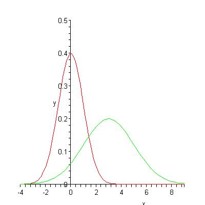
Figure 1
I find (limit to tends to infinity)R/P for the three distributions considered by Deffeyes in his book Hubbert's Peak: Normal (red), Logistic (green) and Lorentzian (cyan). (Lorentzian is also called Cauchy). I won't ask you to read the densities of these distributions in html. Three Normal, Logistic and Lorentzian distributions are plotted in figure 2. I have chosen the parameters mu for all distributions equal to 0 and the other parameters sigma, s and r all equal 1. See my paper for definitions of parameters. Deffeyes has a different and probably better way of choosing values of parameters for comparison in his book.
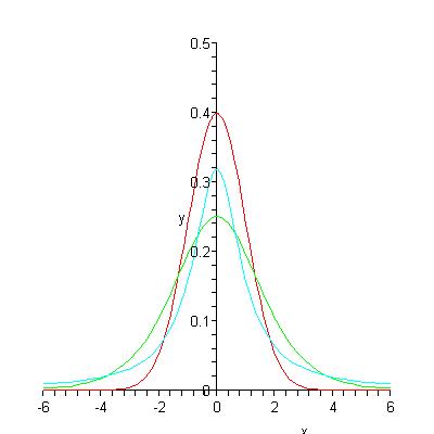
Figure 2
The important observation for our analysis is that the normal density decreases like e-At2 the logistic distribution decreases like e-Bt, and the Lorentzian distribution decreases like C/t2 as t tends to infinity for some positive constants A, B and C. These different behaviours, the "tail behaviours" of the distributions, determine the behaviour of R/P as t tends to infinity.
The main result of the paper is
limit of R/P as t tends to infinity =
- 0 if X is Normal
s(1-e-b/s) if X is Logistic and a=1
as if X is Logistic and a>1
b if X is Lorentzian and a=1
infinity if X is Lorentzian and a>1
Thus, if the distributions are Normal, then R/P does converge to 0. If the distributions are Logistic, then R/P converges to a positive number. If the distributions are Lorentzian, then R/P converges to a positive number or even diverges to infinity. The result for the Logistic distribution when a=1 was obtained previously by Broto in his poster for an ASPO conference .
You can get in touch with me at D.S.Stark@maths.qmul.ac.uk
Personnel
Editors
Contributors
Peak Oil Primers
Archives
- November 2010 (3)
- October 2010 (6)
- September 2010 (4)
- August 2010 (7)
- July 2010 (6)
- June 2010 (7)
- May 2010 (2)
- April 2010 (8)
- March 2010 (4)
- February 2010 (6)
- January 2010 (3)
- December 2009 (5)
- November 2009 (8)
- October 2009 (12)
- September 2009 (6)
- August 2009 (5)
- July 2009 (11)
- June 2009 (8)
- May 2009 (16)
- April 2009 (10)
- March 2009 (7)
- February 2009 (10)
- January 2009 (15)
- December 2008 (9)
- November 2008 (9)
- October 2008 (9)
- September 2008 (13)
- August 2008 (10)
- July 2008 (14)
- June 2008 (23)
- May 2008 (16)
- April 2008 (12)
- March 2008 (16)
- February 2008 (9)
- January 2008 (13)
- December 2007 (13)
- November 2007 (16)
- October 2007 (22)
- September 2007 (8)
- August 2007 (9)
- July 2007 (16)
- June 2007 (8)
- May 2007 (7)
- April 2007 (7)
- March 2007 (10)
- February 2007 (10)
- January 2007 (12)
- December 2006 (9)
- November 2006 (15)
- October 2006 (4)
- September 2006 (5)
- August 2006 (5)
- July 2006 (9)
- June 2006 (5)
- May 2006 (10)
- April 2006 (9)
- March 2006 (13)
Vital Trivia
License

This work is licensed under a Creative Commons Attribution-Share Alike 3.0 United States License.
This post was discussed between TOD contributors, here is a copy of my comments:
It is said that "In order to have a mathematical description of R/P, we must have models of both discovery and production", however discovery does not lead directly to proven reserves. Proven reserves are supposed to represent discoveries that have been developed or are planned to be developed in the near future (let's say within 5 years). The initial discovery strike has to go through some standard oil development phases (decision to develop, planning phase, build phase, etc.) which is introducing a dispersive/smoothing and lagging effect. This relationship between the discovery curve and reserve additions is at the heart of the Shock model. In the proposed approach, reserve is approximated by:
R(t)= CumulativeDiscovery(t) - Scaled_and_shifted_CumulativeDiscovery(t)
It's not clear how good is this approximation.
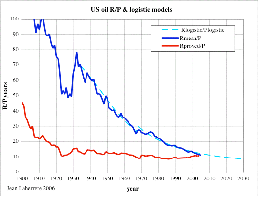
The fact that the R/P is misleading is well known despite being widely used. The best example is maybe the US, where the R/P has been around 10-15 years since 1920:
I think that reserve growth must be important in fact, but what I notice from the paper is the shape of the curves having the effect of interest. Could it not be that what we are seeing there is that each time you calculate reserves, your production rate has also fallen so that the ratio won't converge to zero?
Chris
Good point. I have always said that Production PDF has to be the convolution of a Discovery PDF with some other function. Unfortunately, there is no function that when convolved with another one will give either a Logistic or Lorentzian or Gaussian for that matter. This means that the use of these curves is a contrivance that does not prove anything.
So your point on production rate falling forcing a finite convergence makes a lot of sense because it makes a lot of intuitive sense. It's like pigs sucking out of constantly shrinking trough. The pigs are furiously slurping but as the trough gets smaller, the number of pigs decreases as well.
The convolution of a Gaussian with a Gaussian gives another Gaussian. The sigmas add in quadrature. This is because the product of two Gaussians is a Gaussian and the Fourrier transform of a Gaussian is a Gaussian. It is a special function. I've derived analytically what minimal Gaussian kernels are needed to bring two arbitrarily oriented 2-D Gaussians ellipsiods of differing dimensions into coincidence with the least required distortion to each in an attempt to speed up a program I wrote which derives such kernels for galaxy images obtained with different seeing by means of minimization. The problem there is very degenerate so I wanted to give it a head start. From working on the problem, I can say that you can always take a delta function into another function but after that it gets tricky. Things that look quite narrow sometimes don't have a kernel that takes them into a broader function. But, there is always a pair of kernels that take both into a common function (each other in the trival case) and it is possible to say something about what the best pair looks like.
I think the beginning of the logistics function has a sound basis. If you are making money and you want to make more, you reinvest based on the amount of money you are making. This produces an exponential. The center of the logistics function also has a sound basis: diminishing returns. At some point, putting more effort in isn't getting you anywhere so you put your money somewhere else. I don't know why depletion would look like the logistics function. Perhaps it has to do with wanting to keep some of the people employed who made the whole thing go in the first place. If the coal seam, for example, is running out though, you can only put so many miners at the face. And if an oil well breaks down that is not producing much, you might decide not to fix it. Perhaps depletion is sentimental so it does not get a clear cut off that you might expect.
If you like, I can see if there is a kernel that takes discovery into production via convolution, but convolution is not necessarily the proper method because the time-scale of production probably depends on what has been learned from prior experience. A time varying kernel might be a better representation. It may be possible to take production curves as a function of time and derive a projection that is helpful for estimating the behavior of future or recent discoveries. One catch there though is that the recent curves which are most constraining of future curves may not be complete enough to learn from.
Chris
You are technically correct but this brings up two points:
1. The Gaussian convoluted with a Gaussian is a Gaussian only if it stretches to + and - infinity on the tails. Same thing with a Lorentzian. I see with your background in Fourier optics that this is pretty obvious, but then again spatial diffraction is different than temporal time series in that the former stretches + or - in the limit, whereas temporal has a clear one-sided forcing function due to time causality. (i.e. effects at time at -infinity cannot happen)
So this only means that it is a non-analytic Gaussian and probably approximates it only depending on how bad the temporal tail truncation is. This is even more obvious for Lorentzians convolved with each other, which have even bigger tails.
2. Yet if we may say that it approximates a Gaussian after a convolution with itself, this means that the Discovery profile is a Gaussian! Then we have to explain the rationale for this behavior. And we have another problem to deal with, as we are only switching it from the Production profile to the Discovery profile.
The temporally causal nature of the problem is why I came up with the Dispersive discovery model and the components of the Shock model which use temporally one-sided exponential functions to model the production delays and extraction rates. I am definitely not seeking kernel or windowing functions of the sort you are describing.
I used a simple model, not differentiating between proven and possible reserves, so the analysis would also be simpler. Maybe my analysis could also be applied to your reserve function, but the Shock model described in your link looks a lot more complicated than just using R(t)= CumulativeDiscovery(t) - Scaled_and_shifted_CumulativeDiscovery(t).
Are there models where possible reserves either change to proven reserves or disappear, possibly randomly?
Hi Dudley,
For U.S. oil, the simplest model for the EIA reserves is just 10 times the production in that year. That number is within 20% of the actual reserves for the last 50 years.
For coal, the pattern is different. Countries typically carry unrealistically large reserves, until someone in a resources agency decides that there are no good prospects for new mines. Then the reserves to collapse to the coal that is accessible at working mines. For example, German bituminous coal reserves were reported as 23Gt in the 2001 World Energy Council Survey, but in the next Survey in 2004, they dropped to 183Mt.
Dave
That's interesting. So for oil R/P is about 10 but for coal R/P jumps around. Does it jump around some median value in a white noise or Gaussian kind of way. In Deffeyes' book he uses anthracite coal (I think) as an example which does follow a Hubbert-type curve.
Hi Dudley,
Here is PA anthracite, with the cumulative and the gaussian fits. The reserves are indicated by circles. The reserves are too high, and they do not come down until too late.
Dave
DAve
Interesting that applying the shock model to a Kroneker delta function for a single discovery would add a fixed width production so the scaling on width does not really jive with that model.
In some sense R/P=constant is a pure Markovian rate formulation. The amount of extraction is always proportional to the amount of perceived reserve available. And the reason it starts out high and then damps is because of the transient lags for the shock model phases (decision, plan, build) before the production hits that long-term steady state.
I hazard a guess that this will play out a bit differently using the HSM (Hybrid Shock Model) because the extraction rate builds up with cumulative discovery in HSM. It would be interesting to make the comparison.
Otherwise good use of pragmathematics. Using L'Hopital's rule is indeed clever.
Yes, the scaling on width wouldn't work for a delta function but it could work on a pulse function approximating a delta. The scaling is more about the time delay between discovery and production. It sounds like the Shock model models that time delay in a more elaborate way and is probably more accurate.
The delay and width scaling comes about from convolutions in the shock model. Even taking the Lorentzian example and the Gaussian examples, you get summed (not multiplied) scalings if convolution is at the root. Two infinite Gaussians convoluted together give a new width that is sqrt(w12+w22) and two infinite Lorentzians convoluted together goes as w1+w2. That's at least what I think is at the root of the scalings.
This is a link to a discussion of net exports over on a Drumbeat thread:
http://www.theoildrum.com/node/3529#comment-292688
I am using a modified version of the Reserve to Production Ratio (R/P). I call it Exported Production to Export (EP/E) Ratio. Our (Khebab/Brown) middle case, in our paper on the top five net oil exporters, is that at their 2005 rate of net exports, the EP/E ratio for the top five is 12 years, i.e., at their 2005 rate of net exports, the top five's remaining net export capacity would be depleted in 12 years (2017).
Of course, we don't produce, or export, at maximum capacity and then go to zero in one year, but it gives one a pretty good idea of the problems the importers are facing. Plugging in the expected decline in production and increase in consumption, our middle case shows the top five approaching zero net oil exports around 2031.
Hi Dudley,
Thank you for posting your work. Could you please share with us your thinking on why you used the language of probability theory for this? It is true that fossil-fuel production history often follows a normal curve well. Ken Deffeyes showed us in his books that a cumulative normal curve fits U.S. oil production "like a glove." Clearly the Central Limit Theorem is at work, but how? Production is a time series, which is not the same thing as a probability function. Can you help us out on this?
The other issue, which we have often discussed at the Oil Drum, is that it is not always clear what information we get from reserves. As Jean Laherrere's graph shows, U.S. oil reserves have consistently been about 10 years worth of current production. We get no new information from a number that can be accurately estimated by multiplying current production by ten. He quipped that when the last barrel of oil is produced in the U.S., there will still be 9 barrels of reserves that would then be converted to resources. On the other hand, coal reserves have historically been higher then future production, which means something is wrong with them. Reserves should be a lower bound on future production, and there should be additons over time due to discovery and improved technology.
Dave
Hi Dave,
I used probability theory language because it's what I'm used to, because it seemed natural to express a shifted rescaled function using random variables, and because having amount of discovered oil at least as much as amount of produced oil for any time t corresponds to a property of random variables called stochastic domination. It was not necessary for me to use probability theory language and I did not use any limit theorems from probability theory.
It's fascinating that the normal curve fits oil production, but it's not at all clear how the central limit theorem applies. It's not even clear why the logistic distribution should fit the data. Deffeyes waves his hands a little about applying the logistic equation to finding oil, but, as he says, it's not convincing.
Bentley has a model described in the Strahan book which results in asymmetric depletion curves. I've written a paper about it which has been submitted to a journal. At a Parliamentary meeting on peak oil last week a BP representative said that Hubbert uses a bell shaped curve because of the central limit theorem. Bentley objected to that as well as many other things the BP rep said.
I think looking at simple models can clarify the reasons for a peak and why something like the R/P statistic is nonsense. At the same time, it would be interesting to apply ideas developed for simpler models to more complicated models.
Sorry, I can't help you out with the coal reserves!
Hi Dudley,
Thanks for your comments. Does anyone recall Hubbert mentioning the Central Limit Theorem in his work? My sense is that Hubbert was more comfortable with the logistic function than the normal curve. In his earlier work, he thought in terms of exponential growth, and this made it natural to progress to a logistic function, because the beginning of a logistic function is exponential. Also, before the development of personal computers, the logistic function was much more tractable mathematically than a normal curve.
Dave
We tend to find and--far more importantly--we tend to develop the largest oil fields first. When the large oil fields start declining in a given region, we can't offset the declines with new smaller oil fields.
Caveat is that many things can "fit like a glove" over a certain range.
Thinking in terms of a time-series, the Gaussian or Normal curve has the property of dP(t)/dt = k*(tpeak-t)*P(t) which means that if Production is equal to P(t), then the rate of production is in proportion to the time from initial production. The sign of this rate changes sign at the peak! You have to roll that one around in your mind whether to believe if this is significant to our understanding.
The statistical view of the normal is more difficult since the gaussian tails extend to negative times, which doesn't make pragmatic sense.
The Dispersive Discovery model combines the deterministic time series aspects with a spread of statistical rate values which essentially replace the gaussian formulation with something that makes a lot more intuitive sense.
Hi WHT,
This figure for US oil production is probably one you have seen. The normal curve is constrained to match the actual production in the latest year for which there is data. This leaves only two parameters, a production scale (the ultimate production), and a time scale (the standard deviation), to be determined by a least-square fit. As Deffeyes says, for US oil, it "fits like a glove." And this takes us back to the question about how the Central Limit Theorem is at work.
Dave
Unfortunately it doesn't fit well at all in the first few years after oil was first discovered. That is, the fitted curve also requires a starting point with initial conditions. So a Gaussian actually requires 3 parameters. But it breaks time causality that a time series curve is largely set by the initial values of its data set without a forcing function to drive it. The fit may be impressive but it is more than likely purely coincidental.
As a counter-example, this curve fits much better and it uses really only two parameters, with a starting point fixed in the vicinity of original oil discovery. Notice the strong bending around 1850, something that a parabolic mapping cannot accomplish.

(from the Dispersive Discovery post referenced earlier)
I know that this may all seem a rather intricate argument, but I am after an understanding of what is going on, not some heuristic fit to the data that comes from scavenging through a junk drawer of mathematical curves.
--
I saw a little bit of the PBS Nova show on the hunt for Bose-Einstein Condensation the other day. If you know anything about this topic you find that both Fermi-Dirac and Bose-Einstein become Maxwell-Boltzmann statistics at high temperatures or low concentrations. But the distinctions in the assumptions leading to their derivation make all the difference in the world. It basically explains what is going on at low temperatures and how the properties of BE particles are so different than that of FD particles. And no one would ever make any progress in understanding if you didn't junk FD when looking for the key to BE condensation.
So I argue that we really need to junk the heuristics of oil depletion because no really substantial theory stands behind it.
Hi WHT,
Thanks for showing your very interesting graph again. Your points are well taken. I think that they apply to the future as well as the past, because gaussians roll off faster than in your dispersive discovery model. Would it be possible for you to do a run of historical fits to the ultimate using your model to see how stable predictions of the ultimate have been with time? For comparison here are the historical fits to the cumulative gaussian for US oil. They start to give useful results, within a factor of two of where we are now, in the 40's. The current fit is 225Gb for the ultimate, and it has been relatively stable, but looking at the curves, one could easily imagine it turning up and ending up at 250Gb, which whould be near you. Would your model give a flatter result than this?
I get more stable fits for the ultimate when I fit cumulative curves rather than straight production curves, so it might be worth trying both ways.
The curve labeled reserves is reserves plus cumulative. It is close to the gaussian fit now, but you get the sense that it is correct only in the sense that a clock that has stopped is right twice a day.
Thanks,
Dave
I haven't read up on the Shock or Dispersive Discovery models, but I will just say that my guess is that if there was some nice interpretation of the differential equation for the normal distribution, which is so simple, then it would have been found already. I suspect that differential equations are not the right way to think about the problem.
I've also thought about the fact that the normal approximation doesn't make sense for t before some initial point. One way to avoid that problem might be to note that the normal curve is approximated by Gamma distributions with increasing parameters, and the densities of Gamma distributions are zero on the negative axis. Moreover, the curves from the Bentley model I wrote about above look somewhat like Gamma distributions (but they aren't).
I'll have to read about the Shock and Dispersive Discovery models.
I am putting all my stock in differential equations, and more precisely pragmatic use of stochastic differential equations which are useful for these kinds of problems.
Interesting that the Gamma distribution comes out of the Oil Shock model fairly cleanly, with an order determined by the number of convolution stages you use:
http://mobjectivist.blogspot.com/2005/11/gamma-distribution.html
Like you said it also has the property that "densities of Gamma distributions are zero on the negative axis". See red curve below compared against the Logistic in yellow.

In reality, we don't see the Gamma because the spread in the Discovery profile will wipe out the intrinsic shape. Like the Bentley model you mention, it may kind of look like a Gamma but it isn't.
If you read up on the Dispersive Discovery model and the Shock model, remember that they describe largely orthogonal features of the oil life-cycle. The Shock model requires a forcing function that is provided by the Dispersive discovery model. In other words, the Shock is applied post-discovery.
Also look at Khebab's Hybrid Shock Model, which has the benefit of a somewhat independent take on the original premise. This also tries to unify the Shock model with the conventional wisdom of the Logistic, which is a great service to a more complete understanding of how we have evolved in curve fitting.
Sure I could do this. This is actually a good way to estimate how good a predictor someone has.
Cumulative curves have a built-in filter so I like fitting these better as well. They only suffer from the lack of a good number for the initial cumulative value (since production data is very sketchy early on).
Instead of the stopped clock analogy, it's that everything kind of looks like a Gaussian if it has been convolved enough. It's the understanding of how this happens which piques my interest.
Hi Dave,
I am wondering if the central limit theorem really has relevance. You suggested to me a while back that it might be operating in the many business decisions taken by an ensemble of people, but I wonder if that would be more appropriate to the noise on the curve rather than the curve itself. I can see a large potential for straight determinism rather than a random variable explaining the shape of the curve. In the beginning, money starts to flow so more wells can be drilled. After a while, the edges of the field are found so no more wells are drilled and production levels off until the field starts to be exhausted. Money shifts to discovering new fields once all the wells are built and you have a self-similar process growing until no new fields are found, or, rather, they are found at such a low rate that the discovery effort is considered too expensive.
On coal, discovery is not as difficult so it may not build in the same way. Perhaps production is set more by saturated demand rather than the desire to produce more so that even more can be produced?
Chris
Hi Chris,
Thank you for an interesting comment. To get a gaussian as a deterministic function of time, wouldn't we need to able to interpret the production in terms of the differential equation WHT just gave us in a physical way?
dP(t)/dt = k*(tpeak-t)*P(t)
Dave
Hi Dave,
WHT points to a departure from this form at the beginning, though it would be hard to pick up in fitting without log weighting I think. But, we might try to separate the rate of increase looking like the function iself (exponential) multiplied by a linear term by considering that an oil company reinvesting profits (yielding the exponential) looks like a going concern so that others might get into the game as an increasing function of time. Most folks in the solar industry right now are saying that now is the time to establish market share so there is a rush to get in. Some who are already in are posturing saying that it is already too late and no one can compete with them.
I remember at the time of the peak, oil companies were giving away all kinds of things the way cereal companies do to try to retain market share. Our steak knives at home all came from Shell. The companies would advertize how freindly and helpful their service people were. Now such things seem to only be nostalgic rather than a real marketing effort.
In the function that WHT shows, the decline looks more exponential than Gaussian. The oil companies don't seem to be growing in number now except perhaps very slowly around the Bakken play, so we don't get the extra linear term. So, perhaps we are seeing something physical about how an oil resource that has been exploited in the prior manner drips out its dregs.
This is just a narrative, rather than a demonstration of deterministic trajectory but it points towards the possibility that a random distribution does not underlie the shape of the curve. Rockefeller might be randomly exchanged with du Pont in their businesses but the shape would be the same perhaps.
Chris
"This is just a narrative, rather than a demonstration of deterministic trajectory but it points towards the possibility that a random distribution does not underlie the shape of the curve. Rockefeller might be randomly exchanged with du Pont in their businesses but the shape would be the same perhaps."
I agree "that a random distribution does not underlie the shape of the curve", but I do think that stochastic elements contribute to the profile of the shape. The stochastic elements are basically described by the spread in rates as various reservoirs become discovered and then extracted. The forcing function has some determinism due to the monotonically increasing march of technology and human adoption, which I think completely wipes away any hope that a single random PDF underlies the shape of the curve.
The only caveat is that a convolution of a many gaussians approaches a gaussian due to effects as mdsolar pointed out earlier in the thread. But then again the shock model does multiple convolutions and in accordance to the Central Limit Theorem everything starts to look normal.
It's interesting to consider R/P when a depletion protocol is in place. Suppose it is introduced in a base year when there is apparently 10 years production left and it is decided to extract 10%, 9%, 8.1%.... of shrinking reserves. Under this construction you never quite get to the last drop.
Here P/R = 0.1 (1 - 0.1)^t with limit 0 so R/P is unbounded.
Of course that's true of any exponentially declining function. The limiting factor on oil production is the production cost.
However, net export declines approximate a linear decline--approximately a fixed volume per year that tends to proceed relentlessly toward zero.
I would think that any realistic theory would have near term production as an increasing function of both reserves, and price. If different classes (prices, and well depletion rates) are allowed for presumably as time progresses a greater fraction of production comes from the less desirable wells.
From your description, I think you mean that the amount of production between time time t and t+1 is P(t)=R(0)(0.1)(0.9)^t, where R(t) is the amount of reserves at time t. This makes sense because the sum of P(t) for t from 0 to infinity is R(0). Your P/R ratio is P(t)/R(0).
The actual R/P ratio at time t should be R(t)/P(t). The value of R(t) will be
R(t)=R(0)-(sum of P(k) for k=0 to t-1)=R(0)(0.9)^t. Therefore, R(t)/P(t)=10 for all times t.
This is similar to my result for the logistic equation. The reason R/P converges for the logistic equation is that the tails decay like a negative exponential and here production and reserves decay geometrically, which is the discrete version of negative exponential decay.
I meant logistic function or distribution, not equation.
I agree strongly with Boof in that having a depletion protocol in place means that you can extract a continuouly decreasing fraction of your estimated or perceived reserves available. Which means that R/P can shoot up. Trying to work the math backwards to affect the reserve estimate is not pointing out the real perception of the situation. Oil producers will extract in aggregate a fraction of remaining reserves each year. This is also the heart of the shock model.
The R/P is garbage. Garbage divided by garbage is still garbage.
Khebab makes the point of the US and its static R/P. What about the UK, where according to the BP statistical reveiw, reserves are constant (last year)? With declining production must I really believe that the R/P actually increased? And to cast a nod to Westexas and his ELM, the UK is now a net importer?
I would love to ask Lord Browne why the UK's R/P is increasing when production is declining. These guys are lying to maintain the status quo. We know it and they know it. They know that we know it. But unfortunately all you need to do to maintain the status quo is fool most of the people most of the time.
Lord Browne actually reinforces my belief in peak oil. In 2004 when oil prices were starting to rise, the BP CEO was on national television assuring everybody we would be back to $25 a barrel in the longer term. How long are we going to have to wait?
Gordon Brown was requesting Saudi to increase production at about the same time; they did not. I had a discussion with my boss (just before he retired) with the possibility we may be heading for an oil crisis, he would not wear that one, it was political as far as he was concerned. Oil going to $40 was a real talking point at the time. I am still on my own as a peak oil believer. Its a subject no one will acknowledge as an issue.
My own experience in life is the more corporations deny something, the greater the probability its true!
The "Generally Assume the Opposite" theory, i.e., when a public figure, especially a politician or energy executive, speaks about Peak Oil one should generally assume that the opposite of what they are saying is the truth.
I have run the BP quote through the Generally Assume the Opposite Filter:
BTW, based on the HL models, the ongoing slow decline in world crude oil production relative to 2005 (EIA, C+C) occurred at about the same stage of depletion at which the North Sea peaked (EIA, C+C), i.e. at about 50% of estimated URR.
Westexas,
Don't quite understand whether you support "generally assume opposite theory" or not.
In this instance he (L Browne)seems to be admitting to a supply problem, though in a round about way (as stated he is no longer CEO of BP). In one breath he seems to be accepting there is a shortage ("slow decline in world crude oil production led to higher prices"), in the next we here him say "there has been no physical shortage of oil or gas". Then he goes on to say "rising prices have forced marginal consumers out of the market" which implies there has been/is a shortage (by the fact some users have been forced out). He uses the word "Hope" which is a softening of language used previously. Quoting 40 years L/P is certainly a misleading and does disregard the concept of "Flow" restrictions that will be imposed by the Peak Oil phenomenon.
So I'm confused, has Lord Browne/is Lord Brown changing sides, but slowly?
I have read an article some time ago explaining R/P ratios. I thought then it seemed an absolutely pointless idea. IMO extraction rates and EROEI are all that matter in terms of an energy supply, though in this artificial world of abstract ecomomics, cost matters also. I used to work in the UK coal industry and coal mines use a colossal amount of energy for ventilation, cutting and lifting. In the UK, I have heard it stated that some of the smaller coal mines were operating at negative eroei, but they continued to operate until the late 1980,s. With -ve eroei R/P can still be a large +ve number, but at no net energy. I'm not convinced our politicians get the whole picture. They make so many incoherent policies with regard to energy policy we should not assume they do.
On a light hearted note, on BBC News 24 two economists assured "us" we would not see a recession, only an economic slowdown.
I am the author of "Generally Assume the Opposite."
My version of the BP statement was fiction. I reworded the statement to "Generally Assume" that the opposite of what Browne was saying is closer to the truth.
For example, assume a statement from OPEC:
"We do not have to worry about Peak Oil for decades, if ever. OPEC has significant reserve capacity.
Run it through the "Generally Assume the Opposite" Filter:
"We probably peaked in 2005. No one in OPEC has any significant reserve capacity."
WT,
Sorry for being gormless, I should have read the orginal "again" first! I must admit I did not notice Lord Browne softening when I first read it a day or two ago. My BS detector is usually well tuned to public figures!
So "we will not enter recession in 2008, but can expect an economic slow down with some high street names disappearing"
Filtered=
"2008 could well to be a year of recession with a number of companies failing"
Have I got the gist now?
Bingo.
Actually, I am technically not the author of the theory. Ayn Rand had something like it in Atlas Shrugged--something to the effect that at some point in the story you were able to get accurate news by assuming the opposite of what the papers said.
The R/P is garbage. Garbage divided by garbage is still garbage.
Perhaps it is garbage considering that in empirical terms it is only as good as the data it comes from.
But I agree with Dudley Stark that it has practical significance in aiding to our understanding on how production curves can evolve.