An Oil Production Model from Roger Bentley
Posted by Chris Vernon on August 8, 2008 - 10:46am in The Oil Drum: Europe
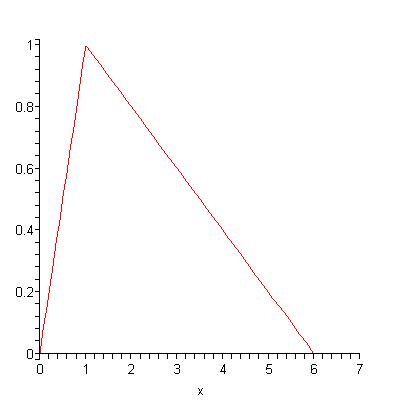
Bentley introduced the following model of oil production on page 204 of Global oil & gas depletion:an overview, and it is dicussed in the book The Last Oil Shock by David Strahan. This posting is meant to explain his model and some results I obtained for it. Consider the following oil production curve:
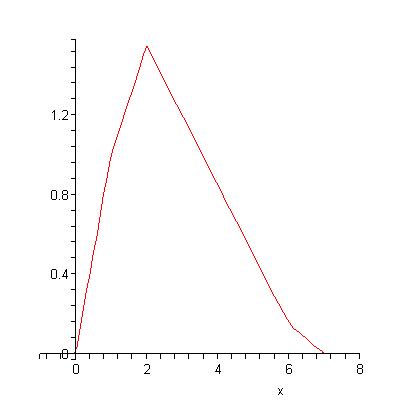
Adding the production of the two oil fields together gives this production curve:
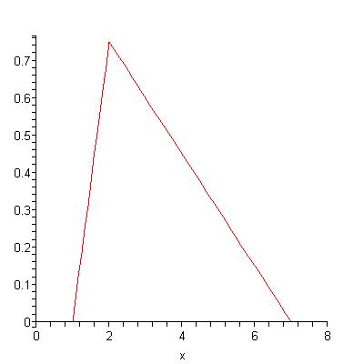
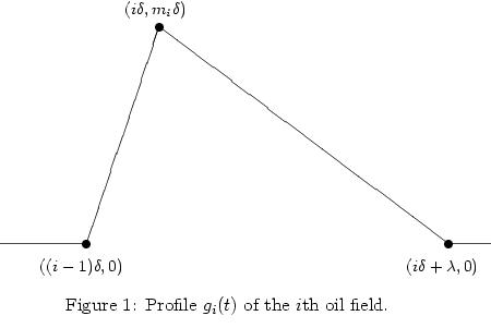
In my paper Peak Production in an Oil Depletion Model with Triangle Field Profiles, accepted to appear in Journal of Interdisciplinary Mathematics, I analyze Bentley's model. The production curve of the ith oil field is assumed to look like this:
I show that in this model, assuming that the mi are decreasing, the resulting total oil production curve is concave on the interval [0,lambda] and is decreasing on the interval [lambda,infinity). The oil production curve therefore takes it's maximum on the interval [0,lambda]. If the mi decrease geometrically, then in addition the oil production curve is convex on the interval [lambda,infinity).
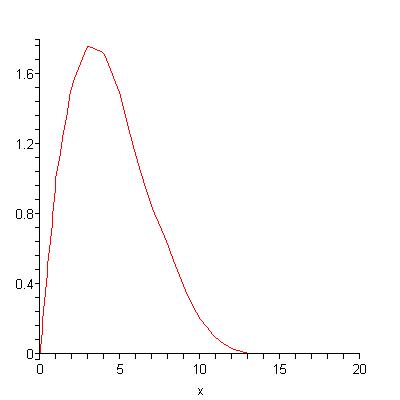
I also show that if delta=alpha/n for a constant alpha and a parameter n and if the mi=f(i/n) for a decreasing function f, then as n goes to infinity the oil production curve converges to a smooth (meaning differentiable) curve which is again concave on [0,lambda] and decreasing on [lambda,infinity). Here is an example of a smooth curve:
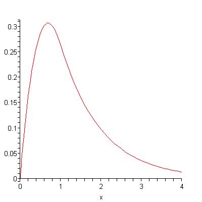
These curves are concave on the interval [0,lambda] and attain their unique peaks there. If f is a negative exponential function (which is the continuous analogue of a decreasing geoometric), then the oil production curves are convex on [lambda,infinity). I show that for these limiting curves it is not possible to have 1/2 of the total oil produced at the time of peak production and in fact they have at most about 35% of the total oil produced at the time of peak production.
A related paper is "Oil Production: A probabilistic model of the Hubbert curve" by Bertrand Michel, who spoke at the ASPO-V conference, to appear in Mathematical Geosciences. In his model the field sizes are chosen uniformly at random from a truncated Pareto distribution. Conditional on the size of the field, the starting time for oil production is Gamma distributed with parameters depending on the size. The field profile shapes are constant; in his application they are given by splines. So Michel's model is similar to Bentley's but harder to analyze and probably more realistic. He uses it to model North Sea oil production (see Figure 11 on page 18). The fit is pretty good except for a decrease in production caused by the "Piper disaster", which couldn't be anticipated by the model.
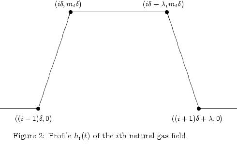
I perform a similar analysis for Bentley's model of gas production, in which the ith field production profile has a trapezoidal shape:
Conclusion
Bentley's model generates plausible looking asymmetric production curves in which less than 50% of the total oil has been produced at the time of peak production. The fact that they are asymmetric is not surprising: see the paper "Testing Hubbert " in which it is found that the asymmetric exponential curve is most often the best fit when six different types of curves are fitted to real data.I'd also like to point out that, though I think papers like this one are important because oil production is important, no one else seems to be doing this kind research in the mathematics of oil production and therefore many math journals wouldn't consider publishing a paper like this. The reason is that they only want to publish papers that reference other published papers in respected journals and this paper only references oil industry papers and peak oil books, as well as another paper written by myself. I was pleased to learn about Michel's paper, which is published in Mathematical Geology, but references a lot of oil industry papers and is like an applied statistics paper.
You can get in touch with me at D.S.Stark@maths.qmul.ac.uk
Previous post from Dudley:
The limit of the statistic R/P in models of oil discovery and production
Personnel
Editors
Contributors
Peak Oil Primers
Archives
- November 2010 (3)
- October 2010 (6)
- September 2010 (4)
- August 2010 (7)
- July 2010 (6)
- June 2010 (7)
- May 2010 (2)
- April 2010 (8)
- March 2010 (4)
- February 2010 (6)
- January 2010 (3)
- December 2009 (5)
- November 2009 (8)
- October 2009 (12)
- September 2009 (6)
- August 2009 (5)
- July 2009 (11)
- June 2009 (8)
- May 2009 (16)
- April 2009 (10)
- March 2009 (7)
- February 2009 (10)
- January 2009 (15)
- December 2008 (9)
- November 2008 (9)
- October 2008 (9)
- September 2008 (13)
- August 2008 (10)
- July 2008 (14)
- June 2008 (23)
- May 2008 (16)
- April 2008 (12)
- March 2008 (16)
- February 2008 (9)
- January 2008 (13)
- December 2007 (13)
- November 2007 (16)
- October 2007 (22)
- September 2007 (8)
- August 2007 (9)
- July 2007 (16)
- June 2007 (8)
- May 2007 (7)
- April 2007 (7)
- March 2007 (10)
- February 2007 (10)
- January 2007 (12)
- December 2006 (9)
- November 2006 (15)
- October 2006 (4)
- September 2006 (5)
- August 2006 (5)
- July 2006 (9)
- June 2006 (5)
- May 2006 (10)
- April 2006 (9)
- March 2006 (13)
Vital Trivia
License

This work is licensed under a Creative Commons Attribution-Share Alike 3.0 United States License.
Chris,
I applaud your effort. I appreciate that you're coming from a math background and not petroleum engineering. I think that allows a useful different perspective. And I suspect you probably understand part of your characterization of a "typical field decline curve" has limitations but I understand modeling needs to start at a simple base and then allow more complexity to enter. Ignoring gas fields for the moment, oil fields tend to fall into two general reservoir drives: water drive and pressure depletion. The build up to peak production results from the time span to bring all field wells online so I skip that section. Your basic model most closely fits that of a pressure depletion drive. As oil is produced the natural gas saturating the oil comes out of solution and aids in the production. But as pressure is drawn down there is less energy to drive the process. But this model is often complicated by the reinjection of produced NG back into the reservoir to maintain reservoir pressure as high as possible. This would alter you basic curve significantly if the pressure maintenance effort is very effective.
In strong water drive reservoirs the oil production rates drops very slowly initially as the buoyancy force of the water pushing the oil up the well bore remains fairly constant. But when the water level approaches the perforations in a producing well the oil rate can drop very quickly. But after the oil/water ration reaches a very low level (let’s say less than 20% oil) the oil decline rate may become very low. I’ve worked with fields that have recovered 100’s of millions of bbl of oil but produced 70% of their cumulative production at oil rates of less than 20% of the total fluid produced. Many of these fields took over 50 years to recover the bulk of their production. Many of these fields are still producing today even though the “oil cut” is down to 1% or 2%.
In applying a model to current global production and looking forward one must look at the drive mechanism of the remaining super fields. Ghawar in Saudi Arabia is a good place to start. Being a strong water drive reservoir its production rate remained fairly level during the early part of its life. But its total production profile is complicated by various secondary recovery efforts including late life horizontal drilling. I can imagine such analysis could be beyond you capabilities. In time perhaps you can have someone with reservoir engineer expertise to assist in this regard. Good luck with your future effort and don’t let the geobabble get you down. Reservoir dynamics are governed by physical laws which lend themselves well to strict math rules.
Ghawar has a reasonably strong water drive, but the early (vertical) wells were so prolific that just a few of them were able to overwhelm the natural water drive.
So, perhaps up to the onset of powered water injection, the depletion profile might be described as suggested by Dudley. After that, however, any simple model might be completely washed out by other factors, including the ones you suggested.
Elsewhere in KSA, maybe the offshore fields, the early fields such as Dammam (shut it after a many years), and Shaybah would be amenable -- although they are injecting gas in the latter.
Interesting post, thanks!
It reminds me what I've tried to do a few years ago:
Convergence of the sum of many oil field productions
I also observed a Gamma distribution:
Some statistical models are also well established in geology such a Lognormal distribution for the distribution of field size. Once the triangle parameters are random variables, the skweness of the resulting production profile almost disappears:
see here for the details.
It's gonna take me some time to digest your article but from a first look it seems that there are no stochastic aspects in your model, the triangle parameters are not random variables, right?
Khebab,
As you probably know log/normal distributions also dominate decline rates for certain reservoir drives. While estimates during the early life stages can be tricky, estimates toward the far end of reserve life become virtually straight lines. Even when secondary recover efforts or additional late life redrilling takes place it usually just represents just an upward vertical shift in the trend with the decline exponent changing very little.
I was actually thinking about the potential of your knowledge base of reservoir dynamics combined with his math skills. It would be interesting to see a stepwise change in his model towards field specific modifications of some of the mega reserves that carrying much of the current output.
If well production profiles is a lot shorter than the total oil production I guess that the shape of the total oil production is almost unaffected by the shape of the production.
The long tail is missing in the production profiles. A simple approximation could be made by making the area of the current production profile a little bit smaller and adding it with a long flat triangle. This a nodal basis and it could be constructed very easy by using two hat functions and a mesh there the points are at the four years [production start, peak, tertiary recovery?, production stop].
From my experience, just getting good info on the value and the time of maximum production per field as well as an estimation of the average decline rate is enough to get a good approximation of the region production profile (see comment on Norway below). Now, you can develop a more sophisticated field model with a production plateau for instance but it does not imporve the result that much and requires much more information per field.
Agree as well. There is something to be said about not overanalyzing a specific region. The macro trends wash out any micro trends as you aggregate these smaller loglet or shocklet functions (loglet is Khebab's idea and I volunteer the shocklet to provide a mnenomic for the oil shock model)
Khebab, I always think of the simplest explanation for a 2nd order Gamma is an exponential damped maturation/reserve growth fuction convolved with a expontial damped extraction function, ala the oil shock model.
I tend to agree. This will likely be the topic of our next TOD press release.
If we're gonna do a press release I'd like to check the math before it goes out.
Deal. As long as I check the spelling.
I agree, it's an elegant and concise solution which has many interpretations.
I do not understand exactly how you and Chris Vernon has done the calculations but I got an idea.
This is the way shold have done it and will if I get enough time:
1. Do an approximation for the distribution of oil field size. Preferably by looking at produced field size in a mature region.
2. Choose a skewed triangle.
3. Let triangle area be equal to field size and delay equal to production year or use the distribution approximation.
4. Sum triangles and plot total production for different triangle skewness.
5. Choose an appropiate skewness (constant or field size or time dependent) and try for other regions.
6. If it works try for world production! and submit result.
I would expect triangle skewness to have effect on total production profile if the quote (field production time)/(region production time) is close to one. It could be a good idea to use well production instead of oil field size because I expect that highly productive well in a new field could be drilled before a low productive well in a mature old field.
The Bentley model has no stochastic aspects. The Michel model has stochastic aspects both in the size of the field and the time production starts, but the shape of the production curve is fixed. Thanks for the link to your work.
I believe the premise missed in this analysis is that field sizes have nothing to do with the shape of the underlying curve. Reading the paper, I would argue that assuming a monotonically declining size of field after the initial discovery is a restrictive constraint. What the distribution in field sizes actually leads to is noise on the curves. i want to point this out because alternative models such as dispersive discovery do not make any a priori assumptions on field size distributions.
Would it be more realistic to keep a triangular curve but let the slopes depend on the field sizes? What assumption does dispersive discovery make? In the Michel paper he comments that he thinks randomness in the total curve is mainly caused by the randomness in the start of production, not in the shapes of the individual curves.
Dispersive discovery assumes a finite volume that is searched. Because of the spread in search rates, it might look as if smaller discoveries are made over time, but that is just an illusion as the slower rates trail the fast ones and lead to diminishing returns as the search space is completed.
One neat part of DD is that in the most general formulation with an exponentially increasing average search rate and exponentially damped search volumes, it exacty matches the logistic sigmoid. I noticed in your paper that you state that 'no interpreation of the logistic equstion to oil production exists'. Well, there you go. Take a look at the derivation, as it comes out quite simply.
What if we were robots, did not have finite lifespans, and did not have evolved wet-ware that strongly favored immediate consumption over delayed reward....
Assume the oil technology we had would be the same as we humans now have. We wouldn't sell the oil - our objective would be to maximize the total amount of oil produced over time (could be a decade, could be a thousand years, whatever time period would maximize Qt)
At what point in the initial ramp up in production, would we use technology to 'slow' down the flow, so as to maximize long term sum of oil extraction?
(Said differently, the modern human system is an economic one. To produce oil we have to buy equipment, labor etc. with money. We need to get a return on this money relatively quickly (time value of money, etc.), so we are eager and willing to let production ramp as fast as it can (barring a complete economic depression.) How much does a positive market discount rate borrow from future production?) (I guess this is more of a geology question than a math question but Im curious if anyone has insight as to the magnitude of this number - is it 1% or 50%?)
Nate. That is an excellent framing device. Putting the greed of humans in the loop allows us to assume that extraction commences as soon as a discovery occurs. The temptation for immediate profit is too great and historically the oil will get 'used' as soon as possible, with little foresight wrt efficiency of recovery.
And as you say, hindsight via knowledge and empirical observations would allow us to manage the full lifecycle much more wisely.
Nate, Hubble
The problem that goes unmentioned in this talk of greed and profit is that our world is essentially a bunch of competing, and at times, warring, tribes. Each tribe correctly perceives advantage in exploiting natural resources aggressively.
Only within an effective world community would such selfish behavior be suppressed.
Given enough time, such a community will emerge. Perhaps it will do so in time to prevent a global energy catastrophe. Perhaps not.
But awareness of the deeper nature of our global predictment is a beginning.
"At what point in the initial ramp up in production, would we use technology to 'slow' down the flow, so as to maximize long term sum of oil extraction?"
typical recoveries from a depletion drive reservoir are in the 10 % range
typical recoveries from a solution gas drive reservoir are in the 15 -25 % range
typical recoveries from a water drive or efficient waterflood are in the 40% range
typical recoveries from gravity drainage are in the 65% range
mother nature works slow, but beats the $hit outta the best laid plans of mice and men.
try this experiment: watch the water drain from the sink when you shave or wash up. and if your plumbing is real new you might hear that sucking sound ross perot spoke of.
there was a discussion a while back about a company's plans to drill incline wells (connected to some sort of tunnel) at the base of an oil reservoir to maximize gravity drainage. this plan was mostly made fun of on tod, but imo the concept has possibilities.
I'm wondering how do oil producers actually balance between maximizing current production and maximizing total oil extracted if more production today means less ultimate production. Does R/P come into it, as Majorian seems to be saying below? Or do producers maximize the present value of the total quantity of oil, with future production discounted by some factor?
"I'm wondering how do oil producers actually balance between maximizing current production and maximizing total oil extracted if more production today means less ultimate production."
the oil producers balance between according to the rule of capture. and mother earth help you if texaco is your neighbor.
that and pw economics.
What is the 'rule of capture'? I've never heard of that. Thx.
rule of capture is based on olde english common law which meant it was legal to capture game that was crossing your land. this concept was adopted and applied in the early days of oil developement(in most u.s. states).
from a practical standpoint, it means that the oil beneath your land, and possibly your neighbor's land, is yours to capture.
the consequences are that companies produce at a maximum rate without regard for total recovery.
texaco, when there was a texaco, had a reputation of ruthless rule of capture practices, alledgedly.
In other words: I drink Your milkshake.
that's right, that's right: i drinka ya milkashaka !!
If you integrate that triangle or sum the cumulative area from left to right you get a pseudo-logistic spline curve. That is a convex quadratic seamlessly joined at an inflection point to a concave quadratic. There's your sigmoid or S-curve which we all agree is the hallmark of increasing returns followed by decreasing returns.
If indeed all-liquids is on a 2005-2008 plateau as suggested on other threads the triangle would seem to have the apex sliced off.
Nice post
No matter how bad a day I have The comment section always cheer me up. Nice info.
David Strahan is a character that deserves a closer look. Why do we keep seeing his name? Who is he?
certainly "ccpo" has asked himself this(these) question(s) every night before beddy byes.
David Strahan is a British science journalist who writes about energy.
His website is here
http://www.davidstrahan.com/index.html
The Depletion Atlas there is fun to play with.
His book is a good read.
I must be extra dense today. This is the second comment I've read that made zero sense to me.
Care to explain?
Best Hopes For Less Confusion,
Cheers
"Just Another Statistic" seems to be a groupie who has latched onto you and is now following you around making asinine and irrelevant comments. You may be amused, having your very own TOD groupie! The rest of us can safely ignore him though.
I don't think so, but I suppose it's possible. The other comment referenced wasn't by JAS, it was by Nate. Nate's reference was obscure, but JAS's is a complete non-sequitur.
Whatever.
Cheers
Dudley, Thanks for this contribution, the most important point being IMO your 35:65 split - to which I will return in a moment.
Rockman makes some good points about engineering - and this brings me to human intervention, technology and economics. A couple of pointers as to how this can modify field production profiles.
When the oil industry moved off shore it became preoccupied with maximising flow rates and cash flow as early as possible - often at the expense of ultimate recovery. 20 odd years ago a company working off shore would install the platform having invested in said platform and often a pipeline too. They would then start drilling wells and bring these on sequentially as fast as they could drill them - always keeping an eye on reservoir pressure to keep this above bubble point. At some point they would have to drill some water (or gas) injection wells for pressure maintenance.
What happened next was that companies started to "pre-drill" wells before the platform was built / installed. So maybe 6 to 10 wells would already be there by the time the steel jacket arrived. I suspect this was made partly possible by low rig rates during the recession that affected the world oil industry from 1980 to 1998. When the platform arrived all they had to do was to hook up the pre-drilled wells and the field would hit "plateau" / peak immediately - pretty like your wedge triangle.
So one thing I'd like to see done here is you playing around with a number of different field production profile shapes - including ones with great long drawn out plateaus like the Saudi supergiants where natural peaks have never been reached owing to conservative field management practices.
Another factor to consider is to compare and contrast field management behavior between onshore and offshore environments. Offshore, fields are inclined to have a more finite life span that onshore - again see what Rockman says. In the north sea for example, the cost of maintaining infrastructure will eventually get too high and it will be decommissioned with recoverable oil still in the ground.
And so to your 35:65 split. This makes intuitive sense to me and helps bridge the gap between those who see a 50:50 split and 2 trillion bbls URR for Earth and those who see much higher reserves - IEA et al. My feeling is that we are in peak oil territory - but according to your model we may still have the best part of 2 trillion bbls to produce. In essence, the post peak decline will be shallow as we (Mankind) do everything we can to wring the last drop out of old fields.
A real world example of this is Ghawar where we have tended to only think about dry oil production and ignore the 10s of billions of barrels that may one day be produced from behind the flood front - that is if the Saudis are in any fit state to make the massive investment to bring this about - which is doubtful for a range of complex reasons.
Personally, I am not bothered about some extended tail for world production that goes on for a long period since I will be dead.
The fall-off to 50% of world peak flow is an almost symmetrical peak! In the real world this means 50% by what date?
A much more important question for me is ... 'What is the split for net exports flows'?
What does the 'net exports' curve look like, when does it get to 50% and when does it get to zero (or very close to it?)? ... and most important of all what will my country be able to sell to buy adequate amounts of those rapidly declining 'net exports'?
In the future more and more oil will come from offshore - experience from the North Sea (where most of my oil comes from) looks more like a 75:25 split at present! ... Unless you believe Gordon Brown's prediction of 25GB yet to find!
Euan,
You’re quit correct about the time factor influence in operational decisions. And, as you point out, it’s all the more critical offshore given the big initial infrastructure costs. Virtually all oil companies adjust for the time factor by using net present value. The common discount rates are usually 15% and as high as 20%. This also takes into account for the production profile. There is a physical limit to high a flow rate any well can maintain without risking catastrophic failure. This is almost always the rate chosen. Usually only infrastructure bottle necks cause lower rates. I’ve seen many commercially producing zones abandoned both off and onshore because a recompletion in a shallow zone has a higher NPV. More common offshore given that the high fixed operating costs are also factored in. And, as you mention, high fixed operating costs will cause an early abandonment.
Back to assumptions of URR vs. the time factor. Onshore oil fields can operate commercially at very high water cuts. There are many fields in coastal TX that are very profitable at 1% oil cut right now. These same fields commonly show a 50% recovery to date. But it has taken 50+ years to reach that level. Most of these wells started cutting water within the first year or so. The production profile is radically different than the common model. Typically 2/3’s of the URR is made at 75%+ water cuts. Applying a NPV calculation using a 15% DR would produce a marginally commercial result for these fields AT THEIR INITIAL PRODUCTION RATES. Yet these fields in this one trend have recovered over 1 billion bo. Now consider Ghawar Field and estimates of URR. Though not an expert on that field I can confidently say it will be producing commercial volumes of oil 100 years+ from today. That volume might only be a few thousand bopd but it will be producing. Only the KSA knows what the current water cut is in the field. But given the nature of water drive reservoirs it’s not difficult to project many billions of bo recovery at the forthcoming high water cut. I bought a field from Shell Oil in S La. that had probably recovered 90%+ of the original in place reserves. Obviously much of this recovery was non-commercial. Why SO continued producing is a long story and not pertinent to the current discussion.
Thus we back to the natural conflict between modeling physically recoverable oil vs. commercially recoverable oil. The physical dynamics of reservoirs are readily projected given enough data base. But actual production profiles will be greatly influenced by commercial and political (why Shell Oil kept producing though loosing money) considerations.
Problem is that this result does not hold on real data. Let's look at Norway's fields:
Approximate them by triangles (The right side of the triangle is not linear but exponential but it won't affect the result):
Sum the triangles:
There is no apparent skewness in the blue curve (I get a 58:42 split), the skewness in the field triangles is so random that the central limit theorem makes any trend disappear.
Khebab,
Excellent.
Your 58:42 split rings a bell, as this was approximately the same split I obtained in some previous work I did
(just need to go through my files to find it.:(
Your curve looks like the exponential fitting curves from the Test Hubbert paper. It seems like randomness can remove skewness and produce a non-Gaussian curve at the same time.
I'd say that overall production is dominated by the largest fields which have a Gaussian like production profile so you don't need to invoke the central limit theorem. Of more interest over the short term is the marginal changes in production from the smaller fields. Splitting production profiles this way is interesting esp if you consider small fields across all producing basins. Although overall production is dominated by the effectively guassian distribution of the largest fields the detailed decline say the first ten years is really controlled by the distribution in small field production levels and time they where brought inline.
Given that historically different regions exploited their smaller fields at different times its not clear what the total effect of the smaller fields are but its a good chance that they have enough of a impact to change the shape overall Gaussian distribution of the larger fields and more importantly the average world production from small fields over time has no reason to be Gaussian as the lifetimes of the fields are not all that different from the rate at which they are brought online in general as fast as one is brought online another one enters decline.
In the particular case of the North Sea the small shoulder about 1995 seems to result from a fortuitous distribution on the smaller fields. Certainly the larger number brought online after 1995 seems to have modified the distribution from a pure Gaussian. World wide depending on how the small fields have been exploited this may be a distortion on the order of 10-15 mbpd from a simple Gaussian.
Deviations in world production of the order of 2-3 mbpd have a significant impact on world oil prices even though they may only be a small distortion of the overall shape.
One data set I'd like to see is the cumulative number of producing oil fields 1900 - 2008 together with the cumulative number of decommissioned fields.
The CERA depletion study showed that around 40% (?) of current production comes from new fields where decline is dominated by expending natural reservoir energy.
Global oil production will end up being dominated by a gigantic stack of old fields producing at 90%+ water cut. We do quite desperately need eroei data on strippers - Nate?
There is always the possibility that it is natural reservoir energy that is key to high eroei and that once that is spent globally it is game over for the human race:-(
It seems like with stripper wells, the real issue is overhead costs and how long the in-place infrastructure will last. Once overhead costs become too high, or the infrastructure (pump or pipeline or something else) falls apart, it is probably game over, because the cost of fixing is too high for the small production involved.
Offshore, stripper wells are much less possible, because of the higher overhead costs. Much of the newer production is offshore. Thus, what we are talking about for stripper wells is pretty much tied to onshore production that is declining.
Does Westexas or Nate or someone have a graph showing the actual curves of former peak areas like Texas, Oklahoma, eastern US and such to use for comparison. To me, the triangle is very front end loaded and that the 35:65 ratio seems too optimistic. I understand ROCKMAN's point about offshore well production peaking almost immediately, but from the North Sea example, I think you still see a less front end loaded triangle and mainly a steeper, shorter time span of the same look, more like Khebab's graphs. I still have alot to learn about how long secondary and tertiary recovery techniques extend field life, but it seems to me that we will tend to sacrifice the tail of production to save the peak if we at all can (atleast until global trade breaks down)
The wedge I believe is back end loaded (for reserves) and 35:65 is a very pessimistic outcome for PO - though not for reserves.
A reserves optimist (3 trillion bbls) who clings to a 50:50 split and a Gausian distribution will see a peak well into the future. This analysis allows the peak to be now. It also makes the status of 1 trillion barrels of reserves highly questionable - very hard to get at oil that may hypothetically be produced between 2050 and 2100 - is not really that relevant to today's debate. Though it may be highly relevant to a world population of 3 billion in 2050 - I'll be 93 years old and am inspired to stick around just to see how this story unfolds.
So I'm clear on what you're saying, are you saying 35:65 to mean 35% of reserves produced to peak, followed by 65% produced after peak and you're saying that is pessimistic (which I would take to mean that you believe the ratio will be more like 25:75 or 30:70)?
When I say front end loaded, I mean the triangle peaks early with a slow decline, whereas I actually believe the triangle peaks more towards the middle or after the halfway (in time) point and decline more rapidly.
Agreed. But the analysis leaves out any mention of EROI, quality, or cost (as it has to, because we don't really have the data). But #barrels * EROI may have peaked long ago (1999?). We could still be getting out 75 mbpd in 2020 but maybe at a 5:1 EROI instead of 15-20:1, implying that if all energy inputs to extraction maintain their same cost proportion to society, oils ability to 'do work' will have been cut by 2/3s.
at 35:65, what is the magnitude of cost increases in the 65? Also, the wells that we can analyze historically were produced during a peaceful globalizing social structure, where parts and expertise can cross borders at will. The downside will be smooth and shallow only if these assumptions hold.
Finally, the 35:65 might work for a well, or several, but to scale up globally does not account for rig limitations etc, that might make the flow rate match up with associated URR - i.e. with 10s of thousands of wells, many may be shut-in until the infrastructure arrives to continue their smooth decline.
The scale does have alot to do with it, along with infrastructural abandonment issues. In theory, one given well can produce tiny amounts for a long time, but the economics of maintaining a 1bbl/d oil well eventually become untenable and so the long tail of 1bbl/d is chopped off. I think that's why this triangle doesn't work, because while technically true, practicality of the energy business changes the actual outlook.
It'd be interesting to make a chart on the EROI of various energy sources from over the years (wood, coal, oil, gas, nuclear, etc). I assume oil would come in at a peak EROI, which means the graph would probably look like a 90:10 triangle of EROI.
If the decline was the result of pressure wouldn't that part of the curve be convex, due to Bernoulli's equation--k*sqrt(P)=Q
(where P is pressure and Q is volumetric flow)?
I would guess that the rate of production in the growth
phase is proportional to the number of wells dug in a field (which is economic) and the cost per well goes down
when more wells are dug. Once the number of wells are fixed it is the extraction phase which would be governed by pressure.
But most models seem to be convex in the growth phase and concave/negative exponential in decline which is different to what I would expect.
At any rate, oil production is an economic activity which is why the deterministic R/P model should work. Economics is about the maximizing production rate not maximizing the resource.
This paper looks a little bit like an opening for Fuzzy Logic (which is an improvement over probability theory?).
http://en.wikipedia.org/wiki/Fuzzy_logic
majorian,
We have to be careful using the term "pressure". In a perfect water drive reservoir the flowing pressure remains fairly constant as the aquifer moves upward as the oil in produced. What eventual drives the oil rate down is the inevitable increase in water production as it reaches the perforations in a well. The total fluid produced will often go up as the effort is made to increase the net oil rate. Towards the end of well life it's not uncommon to see strong water drive reservoir produced 1000 bbl of fluid per day with a 1% oil cut = 10 bopd.
But certain oil reservoirs produce by pure pressure depletion: as production goes forward dissolved NG in the oil is liberated and assists in the recovery. But as you point out, as pressure is reduced so is the driving force. I know of many reservoirs which reached URR at only 10% to 15% because of this effect. These are the reservoirs that were targeted for CO2 injection as well as other repressurizing efforts. The decline curve for such fields will show (after the drill up phase you mentioned) a very linear decrease proportional to the recovery volume. This is why it’s much easier to predict URR from pressure depletion reservoirs than water drive. Water drive recovery estimates will depend on the accuracy of the geologic mapping and a number of critical reservoir engineering assumptions. Or, as we say in the oil patch, with depletion drive reservoirs you see the ball heading for your head. In water drive wells the ball is thrown at you when you’re looking the other way. On the other hand, once you get water cut production for a while it will tend to plot a very linear line on log/normal plots. Even when secondary and tertiary recovery techniques are applied this relationship will generally remain true. Which is why the KSA probably has a very good estimate of the future production curve of Ghawar et al? In addition to having all the detailed data they also have had the best Swiss reservoir modeling engineers in the world working on it for many years.
Are sure they did not have the reservoir engineers producing the best numbers?
karl,
Do you mean inflating the numbers? No...my bet is the engineers are giving the best honest estimate. Now what numbers the SA gov't throws out is a different matter. More times than I can remember I've had my numbers "adjusted" by management because my analysis didn't represent the most "optimistic" interpretaion. That's why these days I always have my copy of a report signed when I deliver it to a client. That way if I ever have to tesitfy in front of the SEC or some angry shareholders I can show what my numbers were before they were "edited". I assume you know how the corporate "Trust me" phrase translates.
Oops.
You're right, of course, that it is much more complex than simple pressure. I was just assuming the rise based on adding oil wells and then when the pressure just starts to drop using pressure to predict output. The curve is convex not concave as seems to be what happens to real oil fields. Is this because they tend to drill too many initial oil wells?
Actually I think that if the goal is to maximize long term output instead of production rate you'd end up with something like a morality curve with continuous pressurizing secondary and tertiary activities adding so many years rather that a given amount of bpd, just as preventative maintenance extends the life of equipment.
The problem with that is that economics not science drives every aspect of oil field use.
Which in a round about way supports the R/P 'economic' model.
majorian,
Too many initial wells? Not too common in the US over the last 40 or 50 years at least due mostly to regulatory restrictions. Overseas I’m not too sure but I would guess not too often. Usually questamites of areal drainage are too optimistic and not enough wells ar drilled. One modification of the model I might suggest: in most cases I’ve studied the drill up phase would be shorter than you show. I’m just eye balling the length of the drill up phase vs. the field life span. Also, your curve reminds me more of an inefficient water drive reservoir (which are fairly common compared to “perfect water drives). While the aquifer does add some support to maintain pressure there is still a limited pressure draw down which does diminish production earlier on. It also looks a little like a combination pressure depletion with some water drive support. That’s probably going to be the most difficult part of your task: there are distinct and different end points to the different drive mechanism and a good bit of overlap. It would simplify the effort if you could categorize the most common drive mechanism within the population you’re working. In other words if you combined two very distinct reservoirs (one a strong water drive and the other a pure pressure depletion) you would end up with a combined model very similar to the one you just posted. And there are many cases in which all the different drives mechanism can be found in different reservoirs in the same field. Thus a field wide model might not fit any of the individual reservoir decline curves very well. This has always been the frustrating aspect of projecting from trend to field to individual well to reservoir. The general assumptions tend to fail more the farther you go down the chain.
"due to Bernoulli's equation--k*sqrt(P)=Q
(where P is pressure and Q is volumetric flow)?"
we generally use d'arcy's law v=q/a =(c*k/u)*(dp/ds)
that sqrt eqn applies to linear flow (as along a fracture) if i remember correctly.
Chris,
Khebab is right. The central limit theorem basically gives you this Bell-curve, even without requiring each oil field to conform to any types of production profile shape. I have pointed out this fact at my own site back in 2006.
http://www.1stmillionat33.com/2006/07/peak-oil/
There is no magic to it. It's just math on random processes.
Regards,
Ok, but i don't see any quantitative info there. no magic, yet no math either.
A couple of comments. One overall the rate at which we bring new fields online is limited by the number of drilling rigs. Offered without proof but overall worldwide then number of active rigs in any given year on average is fairly constant within a reasonable range.
Baker Hughes rig counts from 1975 -2008
http://investor.shareholder.com/common/download/download.cfm?companyid=B...
We see the absolute number change with economic conditions but over the entire production period the number of active rigs is fairly consistent. Certainly details matter but the important point seems to be that world wide production rates at least of the period considered are geared by the number of active rigs and previous production.
If one assumes that in any given year the best fields will be drilled as soon as possible then the wells these rigs drill are biased with both production rates higher earlier on and the lifetime of the well lasting longer earlier on since we always select the largest known field first given the limited number of rigs.
All the data I've seen about actual oil well lifetimes performance etc point to signifcant cherry picking of the best known fields first for actual development next discovery although its fairly random and dispersive seems to lead production by a significant amount. So early on you had a large number of choices to exploit at any given time. As long as discovery can lead production then selection pressure to produce the best/largest fields first seems probable. Well production data points towards systematic declines in productivity increases in drilling depth etc.
Now how to model this ?
I suggest the current paper is pretty close but with some modifications.
First the giant and super giant fields can and should be treated as a different group. The production levels from these fields is significant and accounts for 40-60% of overall production the production profiles of these fields span decades and seem to have a trapezoidal shape consistent in field drilling programs can maintain production levels close to that bottle necked by above ground infrastructure for decades.
Inclusion of production from these fields in global estimates will swamp the production of smaller fields. For most of the production history they can for all practical purposes be considered constant.
Next assuming that the current paper is correct for small fields we need only include the effect of a limit on the rate we can exploit the fields. I think its correct that the bias is towards larger fields first but the peak itself is probably not sharp but a long plateau limited by the number of active rigs.
So a distribution of triangles like this is probably accurate.
2 4 8 16 32 64 64 64 64 32 16 4 2
This is the number of wells drilled or fields exploited the actual triangle dimensions are weighted to the earlier side of the distribution say with a linear weighting with the last fields drilled 50% smaller then the first fields.
What this results in is a distortion of the curve into a sort of shark fin like distribution proably it reaches plateau at 36% but production continues close to this rate well past 50% depletion on finally declining later in the sequence say when we hit the final 16 or 4 fields. The only change is that above ground factors throttle the rate at which new fields can be developed but on the same hand it also allows significant selection for the best fields first as discovery significantly leads development.
The final drop of in production is then driven by the lack of replacement fields and is shaped by the lifetimes of the final fields added. So when replacement stops if the fields have a average lifetime of 10 years production declines rapidly as no fields come on line to replace the previously developed fields and average field lifetime also drops. So assume that not only is the curve weighted best first but also that field lifetimes decline from left to right say from 30 - 5 years.
The move from onshore to offshore advanced in technology etc etc support these sorts of trends.
Advanced recovery and stripper wells adds a small amount with a profile quite similar to the super giants but its quite small and can be treated as a constant with new depleted fields moving to stripper status at a fairly constant rate.
The net result in my opinion is that the final decline curve is heavily influenced by the final decline of the small fields once replacement is no longer possible and should be quite steep. If the super giants decline at the same time then replacement can be assumed to be over for sure as any new fields could only be assigned to offset super giant declines. Without new regions to drill then you see a initial sharp decline from the small fields reaching end of life over a period of the same order of magnitude as the average field lifetime. I think right now thats about 10 years or so.
With an oil field size distribution or maybe "well size".
I posted this yesterday:
1. Do an approximation for the distribution of oil field size. Preferably by looking at produced field size in a mature region.
2. Choose a skewed triangle.
3. Let triangle area be equal to field size and delay equal to production year or use the distribution approximation.
4. Sum triangles and plot total production for different triangle skewness.
5. Choose an appropiate skewness (constant or field size or time dependent) and try for other regions.
6. If it works try for world production! and submit result.
Khebab did a plot yesterday for the north sea and if you look at the middle to the right of this page http://en.wikipedia.org/wiki/Finite_element_method you could see that they use triangles or hat functions as they call them to approximate a function.
It is actually possible to use real data and vary the speed and see how this affects the production curve, what happens if number of wells are constant increase lineary/exponentially. One large problem is how to handle unused fields or wells (constrained production). There should be an approximate equivalence between production and field reserves and size distribution (if your know the field sizes you could calculate the production and the opposite (approximately)).
Oil field size distributions has nothing to do with. Big or small fields can happen at any time. I say this because we should never ignore black swan events and the possibility of large discoveries.
The big fields would tend to get discovered earlier rather than later because they're hard to miss.
And if we're bringing black swans into the model, well, then despite all the apparent hard work that went into it, the model will not remotely represent reality as far as the back side of the production curve is concerned.
Previous historical oil production data are all buffered by the fact that in a scenario where a region was declining, the majority of the rest of the world's oil production was in an upswing, prices were stable, food prices were stable, the climate wasn't shifting, the economy was growing, the population was less into overshoot, and the spectre of war was sporadic.
The black swans of these "above-ground factors" will greatly and negatively impact production, and their effects are not included in the model.
WHT is correct during discovery phase the size the largest fields are not found first but what I'm saying and this seems true from the historical data is that at any point in time we pump the largest fields we know about first and next discovery proceeds development by a significant margin.
The net result is that even though WHT is technically correct we are always selecting for the best largest known fields for development over more problematic or smaller fields.
Look at almost any region. Russia, US, ME. And the discovery phase was able to find and put into production the largest fields quite early in the production history while in general the smaller fields where ignored till later. So in general discovery in a basin is completed enough to detect the largest fields before a significant amount of production is online.
Discovery again becomes important when we move to exploit the smaller fields to make of for declines of the super giants. A perfect example is Mexico with the decline of its super giant it is now scrambling to bring online a number of smaller or more marginal fields to hold production.
If you look at the North Sea data we see the same thing the time when the small fields are brought online is skewed to after the decline of the large fields.
This is REALLY IMPORTANT !!!
The small fields are pumped at a far higher depletion rate vs the large fields production rates are kept high
by replacement i.e as one small field declines a new one is brought online. Once you run out of small fields to add ALL the small field production becomes zero on a short time scale generally 5-10 years.
The world produces between 10-15mpd from the aggregate total of small fields. These fields are being depleted at a rate of between 10-20% ( i.e they have a 5-10 year lifetime) Today we have no way to replace these fields. Depending on exactly how they where brought online this 10-15mbpd goes to zero over the next 5-10 years.
This situation is even clearer for NG. You can split the reserves into conventional and unconventional and on land vs offshore. We obviously extracted the best reserves first.
http://en.wikipedia.org/wiki/Shale_gas
We have know about the shale gas for decades although some of the plays where not completely explored because they where uneconomical until recently. Similar but less clear cut distinctions hold for oil plays.
I've seen Khebab remove reserve additions from the discovery data to recreate an original discovery profile.
All thats required to ensure that we are able to select the best currently known fields for development is that discovery is reasonably ahead of development. I've seen no indication that at any point in time in the past the number of fields being developed in any given year was not significantly less than the number of fields that had been discovered up to that year.
WHT is correct in the big picture sense in that all the discovered oil is eventually developed after some lag and the central limit theorem probably comes into play in the sense that the average delay is a good number.
But this completely misses the underlying bias introduced in development because we had ample information at development time to do selective field development. In fact the development of a lot of oil field technology was driven by the fact that we knew of a number of fields that where not economic with the current technology of the time. Many fields had to be shelved until technology advanced enough to make them economic. The NG shale plays are a shining example of this. And in almost all cases although the technological advancement results in commercially viable flow rates these marginal fields are not equal to previously developed fields.
They either have low flow rates or they have short lifetimes etc.
Have we introduced a significant bias into the global production profile ?
Simply looking at the costs of production today vs past decades using inflation adjusted dollars answers this question with a YES we have.
Sure the super giants will determine the overall production profile for the world but the future of our civilization and lifestyle will be determined by the exact pattern of small field decline. Discovery profiles and the decline of the super giants ensure we are past peak but other than that they are probably not important to our near term future.
We can of course keep publishing pretty symmetric graphs and invoking the central limit theorem to prove how righteous we are but it does not make the answer correct.
Just look at the collapse in production in the shallow Gulf of Mexico. It went of a friggin cliff.
Production? Reserves? Politics?
The distribution over time. The discovery cross-section of big vs small is negligible. All that matters is the progress over a searched volume and the discoveries are effectively randomized. See the noise in the following curve and then consider that when enough samples are taken, all the noise smooths out.
http://www.theoildrum.com/node/3287