Projecting US Oil Production
Posted by Stuart Staniford on January 12, 2006 - 7:59am
 I began a discussion of US oil production in Four US Linearizations, and then continued in Predicting US Production with Gaussians, and Linearizing a Gaussian. This post wraps up my analysis of the US URR (at least for now).
The post that follows below the fold is rather technical, and filled with large images. Here's the executive summary for those who would like to skip the details.
Update [2006-1-13 3:22:37 by Stuart Staniford]: After spending more time thinking during the waking hours, I decided my approach had a flaw, which I've corrected. It changes my URR estimate very marginally from the original 218 ± 8gb to 219 ± 8gb. Details in another update inside the post. Apologies for any confusion.
- I estimate that the ultimately recoverable resource for US field crude production as measured by the EIA will be 219 ± 8gb. Since the EIA believes we've used 192gb so far, the remaining balance is 27 ± 8gb. These are intended as two-sigma error bars, and the figures exclude NGL (see EIA definitions).
- This conclusion come from fitting both Gaussian and Logistic curves to the data in two different ways each, doing extensive stability analysis, and making judgements about the level of agreement throughout the regions of stable prediction in all methods.
- I show that on the US data, Hubbert linearization is the most broadly stable prediction technique of the four I considered (despite the fact that the Gaussian actually fits the data better than the logistic).
- In particular, the linearization is the only one of the techniques considered that has any significant domain of reliability before the peak.
- However, the Gaussian is likely more accurate now that it is well constrained by a long history of data.
- The caveat to this extrapolation is, while these models seem to fit US production amazingly well, we still lack a deep understanding of why this is true. Therefore, there is some risk that the conditions which cause them to fit well might change in the future, thus breaking the projections. I would be surprised if this happens in the case of the US, however.
 Recall that the other day I was making pictures like the one to the right, where I explore what happens when we try to extrapolate US production via a linearization, but we start to mess around with where we start and end the linear fit. The specific one shown is Hubbert linearization of EIA field crude production with linear fit from 1958-2005.
Long experience has taught us that the linearization generally does a bad job in the early part of the history, (though I didn't know why till know) so we don't usually start at the beginning. But then the question becomes how sensitive our answer is to where we start. Deffeyes picks 1958, but why, and is that a good place? Additionally, we'd like to know how sensitive it is to where we end fitting. In the past, we had less data and so had to stop the fit sooner. If our answer has been changing a lot in the recent past, that suggests we wouldn't have a lot of confidence that it wouldn't continue to be volatile in the future also.
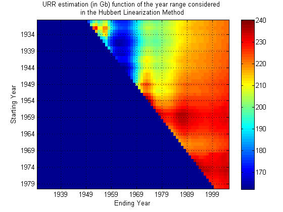 Next, Khebab made the very nice density plot to the right, where he explored a fairly large space of possible starting and ending points. The way to read his graph is as follows. The ending year is on the X-axis, and the starting year is on the Y-axis. For each point on the graph, he has done a linearization, and predicted the final US URR (ultimately recoverable resource). A color-code denotes the answer, and you can see it's been fairly closely around 220gb-230gb for quite a while (the right hand side of the picture), with only modest fluctuations. Encouraging.
I wanted to move the ball a little further down the field. I had two major goals. One was to come up with a quantitative error bar for the URR estimate. The second was to explore which of various prediction techniques does the best job. I noted in a piece on Predicting US Production with Gaussians, that the Gaussian actually fits the US data better, especially in the early stages. Indeed, that seems to be the reason why the linearization doesn't quite work at early times in the production history - the early tail is not matching a logistic well, but is matching a Gaussian well. So I wanted to explore more thoroughly projection with Gaussians too.
|
|
Thus in my analysis I explore predicting URR via four different fit/extrapolate techniques. They are:
- Making a linearization of the data, and then extrapolating the straight line fit out to the X-axis to get the URR.
- Directly fitting a Hubbert peak (first derivative of the logistic) to the production data in the P/t (production versus time) domain.
- Fitting a quadratic to the log of the production data as a way to estimate the Gaussian parameters.
- Directly fitting a Gaussian to the production data in the P/t domain.
These are analagous to Khebab's plot above. Notice that in the far back there is a region where the end year is before the start year, which doesn't make any sense. So I just set the answer to always be zero there. In the foreground of the plots, there is a more-or-less flat horizontal area which I refer to as the zone of stable prediction. Typically it involves having the end time fairly recent, and the start time reasonably early (but the exact nature of the stable region is dependent on technique). As you move around in that area, the answer doesn't change too much. However, as you move back into the plot, things go haywire. The curtain across the middle is the area where the start and end time are a very small number of years apart. Clearly, when that's true, the fit is unlikely to work well as it becomes very susceptible to the noise in the data.
|
|
|
|
|
Now, the most interesting thing to me is that the Hubbert linearization technique (top left) produces the largest zone of stability - there's a noticeably larger smooth area towards the front of the plot, and as it goes haywire towards the middle, it goes less haywire less quickly. The other three techniques are all of roughly similar quality to one another.
This is particularly interesting given that the Gaussian actually models the data better. However, there's a big difference between making pretty fits of past data and actually being able to predict new data robustly. In general, making pretty fits to past data is best served by having a model with a lot of parameters in. That means the curve has more degrees of freedom with which to wiggle itself around to the nicest shape lying along the data. However, lots of parameters means that there are likely to be more different ways that the model can get close to the data, and that allows for greater uncertainty in what the parameters actually are, which allows them to get more wrong. Models with too many parameters can suffer from overfitting in which the regression chooses a model that is essentially optimized to the particular noise in the data, and is losing touch with the true dynamics that would allow it to successfully extrapolate outside of the range where the data is.
A simple model (ie fewer parameters), even if it doesn't actually fit the data as well, may do better just because the few parameters it has are better constrained. The linearization trick has the merit of removing one parameter from the situation (the date of the peak), which then means we are in a better position to estimate the others (at least better when we have only a marginally adequate part of the data history). At least, that's my best guess as to what's going on.
The next four plots are essentially the same thing for the same four techniques, except drawn as contour plots rather than rendered as three dimensional surfaces. This allows us to see what the zones of stability are like a little more quantitatively. In each case, blue corresponds to a URR of zero (or undefined), red corresponds to 300gb or more, and green is the 150gb point. The contours are 3gb apart.
|
|

|

|
So the first thing to become clear again is that the linearization (top left) has the largest region of approximate stability. Most importantly, it's the only technique that is approximately reliable before one actually hits peak (in the mid seventies). J.H. Laherrère in his paper The Hubbert Curve: It's Strengths and Weaknesses makes several Gaussian extrapolations from early on that fail, but here we can see more systematically that the linearization works best for early predictions.
However, another thing becomes clear too - it's stability region is not as flat as the smaller stability regions of the other techniques - in particular the Gaussian techniques. I think what's going on here is that once there really is enough history to constrain the parameters well, the Gaussian technique starts to do better because it is actually a better model of the data. As we know, in the linearization, the early data is always drifting upwards from the straight line, and this tends to distort the estimate unless we make the start date late, and then we cannot take advantage of as much data to fix the parameters as the Gaussian technique can. By using more data, the Gaussian can effectively bridge across the (rather lumpy) noise.
To come up with the URR and error estimates, I took a triangular region at the top left of each picture and grabbed all the different URR estimates out of them. I then got averages and standard deviations of those estimates. I used a larger triangle for the linearization than the other three techniques. Those numbers come out at:
| Case | Triangle side (yrs) | Mean URR (gb) | Edge URR (gb) | Sigma (gb) |
| Linearization | 40 | 215 | 225 | 10 |
| Direct Logistic | 30 | 232 | 236 | 5 |
| Quadratic Gaussian | 30 | 218 | 220 | 4 |
| Direct Gaussian | 30 | 217 | 218 | 4 |
You have to look at these in the context of the pictures above. The linearization URR trend is still going up, whereas the others are flat/wandering as they approach 2005. So I think the linearization is headed up towards the direct logistic estimate of 230gb or so. So the question becomes do we believe that answer or the Gaussian answer. I prefer the Gaussian at this stage, since it's well constrained with this much of the curve in view, and it seems to do a significantly better job of fitting overall, and especially in the early tail. Presumably, there is some central limit type reason for this (though I wish we knew exactly how that worked), and if so, we'd expect the late tail to be Gaussian also.
The main difference in the late tail is going to be as follows. The logistic curve has a decline rate that asymptotically approaches K. The Gaussian has a decline rate that increases at a fixed constant rate per year forever. So in the late tail, the Gaussian starts to decline a lot faster than the logistic. I believe this is why the Gaussian URR estimates are a little lower than the logistic ones.
Given all this, I take as my estimate the Gaussian estimates. What's in the table is the standard deviation, but what I quote above is a two-sigma error bar: 218 ± 8gb. Note, I am intentionally keeping the standard deviation here as the error bar rather than reducing it according to the number of observations since the noise here looks very lumpy rather than iid random. Therefore, I'm not assuming any potential for it to cancel (to be conservative).
My estimate can be contrasted with that of Deffeyes (228gb - based on linearization in Beyond Oil), and Bartlett of 222gb using Gaussians. Also, Khebab quotes a figure of 222gb and has some very interesting discussion but doesn't quote a single error bar. I don't quite agree with his technique there because he's effectively assuming random uncorrelated noise, and the real noise doesn't look like that - it's lumpy and nasty.
Update [2006-1-13 3:22:37 by Stuart Staniford]: I decided on reflection that there's a problem with estimating the URR by averaging over the triangle - it means that the most recent years in the production profile are underweighted in the overall average. Thus we fail to take account of the most recent data properly, which should inform us most. So I added an extra column to the table for the Edge URR, which is just averaged over the leading (most recent) edge of the triangle. I still use the fluctuations in the full triangle for my error bar estimate, however. Otherwise the reasoning is unchanged. So my estimate is now 219 ± 8gb.
Finally, one of the interesting discoveries I made in writing this post was that in making the plot to the right, I actually got very lucky. That is a pretty decent extrapolation that is sitting in a saddle between several areas of quite poor predictions. So sensitivity analysis is always a good idea.
Contact
- Content: editors at theoildrum dot com
- Tech support: support at theoildrum dot com
License

This work is licensed under a Creative Commons Attribution-Share Alike 3.0 United States License.
It would be interesting to see the shape turn from a gaussian curve to more of a steeper drop on the right side.
When people are shown a Hubbert curve for the first time (or second or 3rd) they seem to think that 2030 will be like 1975 which wasnt too bad - but there will be 2.5x the people by then compared to 1975. Just wonder if youd graphically done that before...
-a certainty if we nuke Iran in March.
Teaching differs from simply broadcasting information in that the teacher must modify their behaviour, at some cost, to assist a naïve observer(my edit-me) to learn more quickly.
This is what Franks and Richardson found - follower ants would indeed find food faster when tandem running than when simply searching for it alone, but at the cost to the teacher (my edit-TOD) who would normally reach the food about four times faster if foraging alone.
Journal reference: Nature (DOI: 10.1038/439153a)
Output fell to 4.01 million barrels of oil equivalent a day, 2.2 percent less than the 4.1 million reported in the year-earlier period, London-based BP said today in a statement. BP said it would cut more than 1,000 jobs in Europe to reduce costs.
The Texas City plant, the third-biggest refinery in the U.S., remains closed after a March explosion and damage from the storms and is a setback for BP at a time of high oil prices.
BP said fourth-quarter costs would include $130 million, partly to repair Thunder Horse (my edit-at least $110 m partly and TH doesn't get into the GOM until 07).
So BP's Texas City down, 3 refineries East of NO down along with Pascagoula and the heavy crude Valero plants can't process without hydrogen-the Airgas plant producing the Hydrogen destroyed outside NO.
That's 6 refineries down, still, or producing at much less than capacity.
I saw a short closely cropped video flash by on CNBC/Bloomberg.
If this was TH, the superstructure cranes were crushed into the decking. BP said earlier that TH had suffered 10% damage.
That's how I came up with the $110 million pricetag-10% plus overage.
So many intelligent oil people out there. So little info.
Conoco's 247,000 bpd Alliance refinery is not expected to restart until December or even January
Local environmental activists were alarmed that residents were even visiting the area. EPA tests of the air in mid-September had detected unsafe levels of benzene. "People shouldn't even have been given an option to go back in," says Wilma Subra, an environmental chemist in New Iberia, La., who has served on EPA advisory committees.
Another concern was that it proved difficult to secure it to its anchors in the deepwater current.
(translation: a repeat of 2005 hurricane season in 2006 will cause large approvals of Fischer-Tropsh plants)
I am going to do a quick check on the major 20 or so oil companies in US to look at what they claim to have as proven reserves in US - your analysis assumes we have 218-192 = approx 26 billion barrels left. My gut tells me adding the proven reserves up will be way higher than that.
Which gets back to EROI. Is it possible that one of the mystery reasons why linearization works so well (as compared to other methods) is that it implicitly accounts for eventually reaching a point of EROI of 1-1, even though there is 'oil' left, it just doesnt make energetic sense to get it? Whereas other more aggresssive approaches see 'geologic' oil and just assume it will be pumped?
Hubbert pre-dated EROI but that may be an underlying principle he observed on individual wells and areas.
Incidentally, need I point out that 26 gb doesnt last long when the country in question is using 8gb a year...
Bootstrapping Technique Applied to the Hubbert Linearization
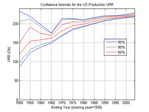
The results are the following for the US production:
larger image
for the [1936, 2004] interval I find the following confidence intervals:
URR(50%)= [220.39 222.65] Gb
URR(90%)= [218.62 225.24] Gb
URR(95%)= [218.19 228.21] Gb
The figure below is the corresponding histogram of the URR estimates from the bootstrap replicates:
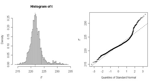
larger image
There is more details in the first link above (with the R source code also). That's it for now, I have to go, I will post more comments later.
In fact, I'm seeing a definite upward trend from 1980 on. I'm not sure that the trend is asymptotic to anything.
Hm, maybe the abiotic oil is seeping in, at a rate that looks like about 750 MB/yr.
YES I'M JOKING!
But something funny is going on.
Chris
Khebab: One rough and ready bootstrap approach you could take is the following. Fit the model to the actual data. Obtain the residuals curve (data minus model). Chop the residual curve up into sections where the end of a section is always a point where the residual curve crosses the x-axis. Thus each section will be a little bump where the data is strictly above the model, or a little bump where the data is strictly below the model. The bumps, I believe, should alternate one up and then one down (some bumps may only have one year in). Now create a series of random permutations of the bumps that preserve the alternating property of them. Create a new replicate by adding this permuted-bump residual curve to the original model. Then fit a new model to that replicate. I believe the permuted bump replicate of the residual curve should have roughly similar autocorrelation structure to the original residual curve. Repeat for many replicates, and use the resulting histogram of parameters for your confidence interval estimation. You'd better actually plot the residual curve, some replicates, and some autocorrelation vs lag graphs and make sure this looks sensible in practice, however.
Another thing that would be worthwhile with your current iid-bootstrap replicates is to do the start-end sensitivity analysis for one of them (since you already have the code). I suspect you'll find the prediction is much more stable than the real data (ie the bootstrap is not producing replicates with enough fidelity to the true bumpiness of the data).
John Fox. Bootstrapping Regression Models, Appendix to an R and S-plus Companion to Applied Regression
I you want to play with the procedure, you can use the R source code (R is a free open source software) I posted on po.com (Bootstrapping Technique Applied to the Hubbert Linearization).
The second procedure in the document - what he calls fixed x-resampling - is what I assumed you were doing last night - taking the residuals from the model, and resampling from those. The issue with applying bootstrapping here - under either of those approaches - is that because the resampling is independent, the fluctuations it introduces relative to the original data have no autocorrelations year to year. Hence these fluctuations are very unlike the original noise. In particular, they are likely to move the regression fit around less. The original noise, because it is quite autocorrelated (bumpy) can have multiple years conspire together to throw the prediction off. The deviations from the model introduced by the bootstrapping do not have this property.
I suggested my residual-bump-permutation idea because it seems to me the resulting replicates would have the right kind of time structure (lumpiness), but preserve the non-parametric sampling aspect that is so attractive about bootstrapping. I could be wrong though - it's just an idea at this point.
Thinking about it now, if you construct the sequence of residual bumps, you could also resample from those, instead of permuting them. I doubt it would make much difference either way.
That's correct. I didn't have a chance to look at the fix x-resampling yet. I don't know if iid noise is a requirement of the bootstrapping approach. My guess is that it's not a requirement because the method is a non parametric way to evaluate the error pdf. If I understand correctly you are proposing a non uniform resampling to take into account the noise "bumpiness".
Does that more extreme example make the general issue clearer?
There is also maybe another phenomenon when we do the following regression:
P/A= aQ+b
then we estimate the URR:
K= -b
URR= -b/a
The URR will be dependent on the error (bias and variance) on both a and b. Put another way, there is a negative correlation between the estimates for K and the URR. For instance, the figure below shows a catterplot of the bootstrap replications of the URR and K coefficients for the BP data (the concentrations ellipse are drawn at 50, 90, and 99% level from the covariance matrix of the coefficients):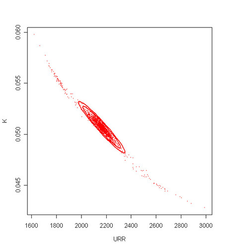
In particular, if K is overestimated post-peak then the URR will be underestimated and conversly.
Not necessarily, any estimator has a bias and a variance that hopefully converge toward 0 when the size of the dataset increases. We can see clearly that the estimator variance is going down with time.
The requirement for a gaussian seems to be a lot of identical and independdent production profiles. I started a little experiment on peakoil.com about that (Convergence of the sum of many oil field productions). If the production profiles are not identical (random URR, depletion rate, growth rate), the curve becomes skewed and has a tendency to become a Gamma function (the gaussian is actually a special case of the Gamma). Part of the answer lies in the Central Limit Therorem convolution formulation or equivalently in the manipulation of the characteristic functions (fourier transform of a pdf).
- The sum of N logistic functions is supposed to be what? a Gaussian or a new Logistic?
- What made you assume the production of a single field to be a traingular distribution function? Can you reference some work on single field production?
Thanks, and keep up the good work.I looked at your 3D surfaces and I'm not convinced of that. For the Hubbert linearization, the domain delimited by the end year > 1990 seems very flat and stable to me. I you take the line of URR values for the end year equals to 2005, it's a very flat line compared to the other methods which have a bumpy behavior when start year > 1975. Because the Hubbert linearization increasingly dampens the effect of noise for mature years (>1975) the fit will always be more robust for ending years > 1975. Too bad, we can't perform a gaussian fit in the P/Q vs Q domain to see how if this effect benefits also to the gaussian.